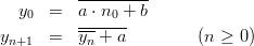
Definition 1.1 Let a,b,y0  ℤM. The linear congruential generator
(abbreviated as “LCG”) with parameters M,a,b, and y0 defines a sequence (yn)n≥0
in ℤM by
ℤM. The linear congruential generator
(abbreviated as “LCG”) with parameters M,a,b, and y0 defines a sequence (yn)n≥0
in ℤM by

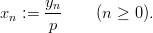
and a sequence (xn)n≥0 of pseudorandom numbers in [0, 1[ by
Explicit Inversive Pseudorandom Number Generators
Diplomarbeit
zur Erlangung des Magistergrades
an der Naturwissenschaftlichen Fakultät
der Universität Salzburg
eingereicht von
Otmar Lendl
Salzburg, im November 1996
As a rule, random number generators are fragile and need to be treated with respect. It’s difficult to be sure that a particular generator is good without an enormous amount of effort in the various statistical test.
The moral is: do your best to use a good generator, based on the mathematical analysis and the experience of others; just to be sure, examine the numbers to make sure that they “look” random; if anything goes wrong, blame the random-number generator !
– Robert Sedgewick, in “Algorithms” (Second Edition, 1988)
I’d like to thank everybody who helped to make this thesis become reality. Peter for his patience, trust and guidance; Charly, Hannes, Karin, and Stefan for the most creative, helpful and entertaining working environment I have ever experienced; and my mother for her unwavering support.
The purpose of this thesis is to discuss the implementation of the explicit inversive congruential generator (EICG) and the properties of the resulting pseudorandom numbers. But before we delve into the details of the implementation or the theoretical and empirical results we will take a closer look at the basic concept of pseudo-random numbers.
What do we mean when we talk about pseudorandom numbers (PRN) ? And for what purpose do we devise such elaborate means to artificially generate megabytes of digital noise ?
To the uninitiated, all this pseudo-random numbers “business” seems to have no serious applications. Everybody will come up with computer games as a field where pseudo-random numbers are used to make the behaviour of the computer less predictable. Steering the movements of some on-screen monster does not require a high standard of randomness, almost any algorithm will suffice, provided it is easy to implement and does not cost too much computing resources.
Another domain where we need PRN is wherever we need to model a more or less random phenomenon of the real world. The simulation of a roulette table or other forms of lottery might still be in the area of non-serious application, but here the defects of the generator start to be an issue. Imagine this scenario: you try to develop a winning strategy for blackjack and use a simulation to test your algorithm. Any correlation between statistical defects and the strategy will lead to a skewed result and may even change the sign of the expected outcome. Playing that strategy in a real casino might cost you dearly. Thus it is important to make the choice of the generator an issue even in such non-scientific applications.
Simulation of random events is far from being limited to gambling, a significant percentage of all simulations of natural phenomena contains a random component. Whether that may be quantum effects, rainfall on a certain area, Brownian motion, absorption pattern, bifurcation of tree roots, failure of technical components, solar activity …, in all cases we know at best the statistical properties of an event. An analytical solution of the given problem based on probabilities is often not possible. Thus one has to resort to stochastic simulation (see [3, 48, 75]) where one calculates the result of the overall simulation by choosing possible outcomes of the underlying random events according to their respective probability. Doing this a number of times should provide enough samples of the outcome to estimate the probability of each possible result. Needless to say, the selection of the realisations of the underlying random events is crucial to the correctness of the whole calculation. Since this selection is done with the aid of PRN, their quality plays an important role in the whole process.
Finding the use of PRN in stochastic simulation is not that surprising, but finding them in algorithms for such mundane tasks like integration might need some more explanation. Numerical integration is a common problem in a great deal of real world problems. A big battery of algorithms (trapezoid method, Simpson’s method, spline quadrature, adaptive quadrature, Runge-Kutta, …) was developed to minimize the calculation costs while increasing the accuracy of the result. All these methods scale very badly with the dimension of the integral, so a completely different approach is more appropriate there. The Monte Carlo method (see [3, 48, 78, 84]) uses randomly selected samples of the function to estimate the integral. Provided we know more about the behaviour of the function (i.e. its total variation) and the distribution of the actual samples used (as measured by their discrepancy), the inequality of Koksma-Hlawka (See page §, [51, 70]) will give an error bound for this method. Since it is generally not possible to calculate the exact value of the discrepancy of the random numbers used for the integration, this error bound will only be a probabilistic one. In order to get a deterministic one, the random numbers, which determine which samples of the function will be evaluated, are replaced by numbers for which the order of the discrepancy is known. This turns the Monte Carlo method into the Quasi-Monte Carlo method.
One way to get such good point sets is to explicitly construct them with that goal in mind (See [70] for a discussion of (t,m,s)-nets and other methods.) or use a PRNG for which an upper bound on the discrepancy is known. This is one of the reasons why we will take a close look at this quantity in Section 3.3. Not all applications of Quasi-Monte Carlo integration are labeled as such, as the basic algorithm can be regarded as a simple heuristic. For example, distributed ray tracing [32, p. 788] uses a set of randomly distributed rays to implement spatial and temporal antialiasing which amounts to an integration over both the time-frame of the picture and the pixel’s spatial extension.
Non-deterministic algorithms often use pseudorandom numbers, too. These algorithms are used to tackle problems for which a deterministic solution takes too much time. Although they cannot guarantee success, they promise to find the solution (or a sub-optimal one) within reasonable time. Examples for this kind of algorithm are Pollard’s rho heuristic [8, p. 844] for integer factorization, the Rabin-Miller primality test [8, p. 839], Simulated Annealing [31], and Threshold Accepting [11].
Other algorithms use pseudorandom numbers for a different purpose. Instead of using them directly for solving the problem they are used to randomize the problem (or the algorithm) in order to avoid running into the same worst-case behaviour again and again. See [8, p. 161] for an explanation of the rationale behind randomized quick-sort.
Some cryptographic algorithms and protocols require a good source of random numbers, too. Stream ciphers [77, p. 168f], for example, use the output of a PRNG (termed keystream generator) to encrypt the plaintext. The security of this cipher depends largely on the statistical quality of the keystream. Any regularities of the PRNG can be used by the attacker to predict the next bits and thus crack the code. No other domain of PRNG applications has such a high demand on the “randomness” of the generated PRN. Algorithms which are good enough for stochastic simulations are typically way too predictable to be useful as a keystream generator for a stream cipher. Thus the field of cryptographically secure PRNG has amazingly little in common with the study of PRNG for stochastic simulation on which we will focus in this thesis. Information on cryptographically secure pseudorandom numbers can be found in [52], [82], and [77].
Another application of pseudo-random numbers in the field of cryptology is providing the “random” numbers needed for a variety of cryptographic protocols. A well known example are the session keys generated for each transaction in hybrid cryptosystems. As the recent debacle involving the Netscape Navigator [33, 69] has shown, one must be very careful not to use a simple PRNG for this task. Since this is more a matter of how to get the entropy needed for non-predictability than one of analysing the properties of sequences of PRN we will not elaborate on this subject in this thesis.
Now that we know a bit about the various applications of PRN, let’s try to formulate a few criteria for the selection of a good PRN generation algorithm. As we will see later it is crucial for the selection of the right PRNG to keep an eye on the application of the PRN.
This criterion may sound strange at first sight, since reproducibility contradicts the intuitive notion of randomness, and indeed, real random number generators are extremely unlikely to ever repeat their output. So what are the advantages of a generator which will produce the same sequence of pseudorandom numbers when fed with the same parameters ? Once again, we have to turn to the application of which the generator is a component. In the case of a stochastic simulation the benefit is twofold:
In some areas, for example stream ciphers, reproducibility is a key requirement for the application. Only very few applications, most of them in the area of cryptography, do actually benefit from the use of non-reproducible PRN.
It is clear that when we want to simulate a random variable with a PRNG, then the output of the generator should model as closely as possible the expected behaviour of instances of the random variable. If a simulation of a dice generates a 7 or strongly favors the 6 we will not accept the generator. Other deviations from the desired behaviour, e.g. correlations, are harder to detect, and methods for systematically testing generators for such deficiencies have been the subject of considerable mathematical work [50, 28, 54, 85], including some parts of this thesis.
As we will see later, proving that a generator really has all the statistical properties a real random number generator is supposed to have, is not possible. So all we can do is to establish faith in the generator by testing it for some properties.
Empirical testing usually involves using the PRN for a stochastic simulation with a known result. If the computed results contradict the expected ones, the generator will be dismissed as not suitable for that kind of stochastic simulation. A passed test will increase the faith that this generator will yield correct results in real world problems. We will examine the significance of empirical test results later in greater details.
A large battery of such tests was developed over the years, from the well known tests of Knuth [50] and Marsaglia [66] to recent additions like the weighted spectral test [40, 41, 46, 44]. See [54, §3.5.] for further references on testing pseudorandom number generators.
In order to make analytical investigations possible, most modern PRNG are defined in quite simple mathematical terms. It is a tradeoff: The simpler the algorithm, the easier it will be to prove statements concerning the quality of the generated numbers. On the other hand, a convoluted algorithm appeals to the intuition. History has shown [50, 74] that quite a few people could not resist the temptation to build generators based on doing obscure transformations on numbers stored in computers. Empirical analysis has shown that the quality of such generators are often abysmal.
Doing empirical studies on the properties of a PRNG is always possible, but deriving properties of the generator output by pure mathematical study has a lot of advantages. Whereas an empirical test can only cover one specific set of parameters of a generator, it is sometime possible to make analytically proven statements on the properties of PRN generated by a certain generator regardless of the parameters used. In the same vein, an empirical test on a specific part of the generator’s output, say the first billion numbers, may give us confidence on the behaviour of the next billion numbers, but cannot offer any guarantee that they will be equally good. Analytical results fall in the following categories:
For most generators not all possible parameters will result in a functional generator. A typical question is that of gaining the largest possible period length. For the LCG1 this is just a set of simple conditions, for the ICG it involves finding IMP polynomials [6, 30, 45, 42, 43, 25]. For compound generators to work it is also necessary to obey certain analytically derived constraints.
For some generators it is possible to derive statements on some aspects of the output. The well-known fact that tuples of LCG generated numbers form lattices (see page §) is one example.
Especially the discrepancy has been the subject of analytical study. There are numerous estimates and bounds for various generators.
With all the mathematical discussions about the merits of PRN generated by a new algorithm one should not forget the fact that we need to actually implement this algorithm on a real computer. There are a few things which should be noted here:
Implementing (i.e. programming) an algorithm is usually a one-time investment of effort. Once the code is there, integrating it into a larger project is more or less trivial. What are the difficulties in implementing a typical pseudorandom number generation algorithm ? As we will see later in Chapter 5, the main problem lies in the handling of large integers and performing standard mathematical operations like addition and multiplication on them. For inversive generators finding the multiplicative inverse in ℤp* is a required operation, too.
The execution of any algorithm requires both CPU and memory resources. Typical PRNG (EICG, LCG, ICG, …) have only very small memory requirements. The code is very compact and the state information does only require a few bytes.
As far as CPU consumption is concerned, a PC with Intel 486DX2-66 processor is capable of executing the EICG algorithm about 70000 times in a second. The author’s implementation of the LCG runs at about 400000 PRN per second. The highly optimized system pseudorandom number generator runs at over 700000 calls per second. These numbers are only provided to give a rough feeling for the speed of the algorithms when using a modulus in the range of 231.
As the generation of the PRN is usually performed on demand on the same computer as the stochastic simulation for which they are used, they compete for the same resources. The total running time for the simulation can be described as the sum of the time used for the PRN generation plus the time used for doing the actual calculations. The latter often dominates the former, thus it does not make sense to try to gain overall speed by sacrificing quality in the PRN algorithm.
After implementing the algorithm one has to find good parameters for that generator, too. Fortunately, for some common PRNG tables containing suitable parameters have been published [29, 43, 2, 83], so there is no need to reinvent the wheel there. Other generators like the EICG are known to be rather insensitive to the choice of the parameters.
Another aspect is the possibility to generate independent streams of pseudorandom numbers. Such streams are needed for parallel or vectorized computing. See [55, §8], [1], [12], and [36] for more information on this topic.
There is no shortage on proposed pseudorandom number generation algorithms. Every year new ideas on this topic are published, but only if the resulting PRN have been subject to intensive theoretical and empirical study the generator might have a chance to get used in a real world problem. As it is often the case with competing inventions, an objective technological superiority does not immediately lead to market domination. Whether the generator is included in standard programming libraries seems to be much more important than any published results on the distribution properties of the numbers. A classic example is the now infamous RANDU generator which was included in IBM’s Fortran library and features an extremely poor distribution of triples composed of subsequent numbers.
The following list introduces some of the most commonly used generators as well as the inversive generators on which we will focus in this thesis. More complete surveys on the current menagerie of PRNG can be found in [70, 72, 55].
In the following M denotes a positive integer (termed modulus) and ℤM = {0, 1,…,M - 1} represents the system of all residues modulo M. With the addition and multiplication modulo M the set ℤM acquires the algebraic structure of a finite ring. If the context makes it clear that we operate in the ring (ℤM, +,⋅) we will omit the trailing “mod”.
Definition 1.1 Let a,b,y0 ℤM. The linear congruential generator
(abbreviated as “LCG”) with parameters M,a,b, and y0 defines a sequence (yn)n≥0
in ℤM by
and a sequence (xn)n≥0 of pseudorandom numbers in [0, 1[ by
As the sequence lcg(p,a,b,y0) = (yn)n≥0 is defined by a recursion of order one on a finite set it must be periodic. The longest possible period length is M in the case of b≠0 and M - 1 in the case of b = 0. The necessary conditions for achieving these period lengths are well known. [70, p. 169]
The LCG is very popular. Its implementation is quite simple, especially if M is chosen as 2 to the power of bits per native word of the computer (e.g. 232) which reduces the modulo operations to just ignoring the overflow. Due to its simplicity and popularity the LCG has been subjected to intensive analytical and empirical examination. The quality of the resulting PRN depends very much on the choice of the parameters M,a, and b. Fortunately, tables containing good parameters have been published, see [29, 27, 53].
The output of a LCG shows a strong intrinsic structure ([65], see also p. §). A number of modifications were proposed to improve the quality of the generator. One approach is to extend the recursion to higher orders by making yn a function of yn-1,…,yn-r. Other proposals modify the function which describes the recursion. As the name says, the LCG uses the linear function f(yn) = a ⋅ yn-1 + b (mod M) to calculate yn from yn-1. If we replace f by an arbitrary function, we refer to the resulting PRNG as a general first-order congruential generator [70, p. 177]. In order to guarantee maximal period length, the function f must be carefully selected. For example, the quadratic congruential method, as proposed by Knuth in [50, §3.2.2] uses a polynomial of degree 2 as the recursion and a power of 2 as the modulus. See [70, p. 181f] for the conditions on the parameters and analytical investigation on the resulting PRN.
Shift-register generators differ from standard linear congruential generators in two respects. First, they use a higher-order linear recursion of the form
 | (1.1) |
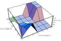
where M ≥ 2 is the modulus, k ≥ 1 is the order of the recursion and a0,…,ak-1 are elements of ℤM. Second, instead of just scaling the yn to the unity interval to get the pseudorandom numbers, the xn are calculated from a block of consecutive values yn,…,yn+m. Thus it is no longer necessary to use a large modulus to get a decent resolution of the resulting PRN. In order to simplify and optimize the implementation of recursion, the common choice of M is the prime 2. On a L-bit computer this allows the grouping of L steps into one operation.
Two techniques for the transformation of the sequence (yn)n≥0 into a sequence of pseudorandom numbers in [0, 1[ are commonly used: The digital multistep method puts
 | (1.2) |
The Tausworthe generator [81] is a special case of this method.
More popular is the generalized feedback shift-register method (GSFR) which can take advantage of the above mentioned blocking of L bits if h1,…,hm ≥ 0 are selected suitably:
 | (1.3) |
If the parameters are carefully selected the period length will in both cases be per(xn) = pk - 1.
Shift register pseudorandom numbers have the advantage of a fast generation algorithm and a period length independent of the limitations of the integers used for the calculation. See [70, Chapter 9] and [55] for a discussion on the properties of shift register pseudorandom numbers.
A promising modification of the LCG was proposed by Eichenauer and Lehn in [14]. We will only consider the case of a prime modulus p = M here. It involves the operation of modular inversion in ℤp which we will denote by an overline (c).
 | (1.4) |
The restriction to prime moduli guarantees the unique existence of an inversive element in ℤp. This definition implies cc ≡ 1 (mod p) for c≠0.
Definition 1.2 Let p be a (large) prime and a,b,y0 ℤp. The inversive
congruential generator (abbreviated as “ICG”) with parameters p,a,b, and y0
defines a sequence (yn)n≥0 in ℤp by

and a sequence (xn)n≥0 of pseudorandom numbers in [0, 1[ by
Empirical as well as analytical investigations indicate that the output of an ICG is superior to the output of a LCG in several respects: longer usable sample sizes [85, 61], less correlations between consecutive numbers [72].
Analytical calculations have led to the following observation: We can describe the
generator as a function mapping n to yn. This self-map n yn in the finite field ℤp can
be written as a uniquely defined polynomial g with degree d < p. If we demand the
sequence (yn)n≥0 to have the maximal possible period length p, the polynomial g maps
ℤp onto itself and thus must be a permutation polynomial, which is either linear
(d = 1) or satisfies 3 ≤ d ≤ p - 2 according to [64, Cor. 7.5]. It turns out that the
degree d plays an important role in the analytical examination of the generator in a
sense that a higher degree seems to indicate better distribution properties [70,
Theorems 8.2, 8.3] (see p. §). The theorem of Euler-Fermat tells us that evaluating
cp-2 corresponds to the calculation of the multiplicative inverse. In this spirit, the
definition2
of the EICG seems quite natural:
yn in the finite field ℤp can
be written as a uniquely defined polynomial g with degree d < p. If we demand the
sequence (yn)n≥0 to have the maximal possible period length p, the polynomial g maps
ℤp onto itself and thus must be a permutation polynomial, which is either linear
(d = 1) or satisfies 3 ≤ d ≤ p - 2 according to [64, Cor. 7.5]. It turns out that the
degree d plays an important role in the analytical examination of the generator in a
sense that a higher degree seems to indicate better distribution properties [70,
Theorems 8.2, 8.3] (see p. §). The theorem of Euler-Fermat tells us that evaluating
cp-2 corresponds to the calculation of the multiplicative inverse. In this spirit, the
definition2
of the EICG seems quite natural:
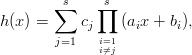
Definition 1.3 (Eichenauer-Herrmann [15]) Let p be a (large) prime and
a,b,n0 ℤp. The explicit inversive congruential generator (abbreviated as
“EICG”) with parameters p,a,b, and n0 defines a sequence (yn)n≥0 in ℤp by

and a sequence (xn)n≥0 of pseudorandom numbers in [0, 1[ by
As long as a≠0 this generator will always have period length p. Once again analytical and empirical investigations have shown that the output of this generator is superior to that of an LCG. This will be the generator on which we will focus our attention in this thesis. The other generators mainly serve as a reference against which the EICG must compete.
Two variations of the basic explicit inversive congruential generator have been proposed. Both proposals substitute the prime modulus p with M = 2ω (ω ≥ 4). In the set ℤM we can define the modular inversion only for odd integers. This inversion is once again defined by cc = 1 (mod M) for all odd c.
Definition 1.4 (Eichenauer-Herrmann and Ickstadt [22]) Let M be a power of
2, and a,b,n0 ℤM with a ≡ 2 mod 4 and b ≡ 1 mod 2. The explicit inversive
congruential generator with power of two modulus with parameters p,a,b, and n0
defines a sequence (yn)n≥0 in ℤM by

and a sequence (xn)n≥0 of pseudorandom numbers in [0, 1[ by

The conditions on a and b guarantee that the sequence x0,x1,… is purely periodic with period M∕2. While powers of 2 as modulus have certain advantages for the implementation of the generator, all theoretical investigations [22, 16] on the quality of the resulting numbers have concluded that this generator is inferior to the original EICG.
In order to achieve a period length of M, Eichenauer-Herrmann [17] proposed the following generator:
Definition 1.5 Let M be a power of 2, and a,b,n0 ℤM with a ≡ 2 mod 4 and
b ≡ 1 mod 2. The modified explicit inversive congruential with parameters p,a,b,
and n0 defines a sequence (yn)n≥0 in ℤM by

and a sequence (xn)n≥0 of pseudorandom numbers in [0, 1[ by

Although this modification does indeed increase the period length to M, the theoretically derived properties of the resulting numbers are still inferior to the original EICG.
An interesting meta-generator is the compound method. This is a very simple and effective way to combine several streams of PRN into one single sequence with (hopefully) superior properties. It works as follows: For 1 ≤ j ≤ r let x0(j),x 1(j),x 2(j),… be a purely periodic sequence of pseudorandom numbers. Then we get the compound sequence x0,x1,… by
If the subsequences are purely periodic with distinct period per(xn(j)) = p j, then we have per(xn) = ∏ j=1rp j.
This compound method extends the well-known approach of Wichmann and Hill [88]. The properties of the resulting sequence has been subject to a number of publications; we refer to Niederreiter [72, 4.2] for all the references. Generally speaking, the compound method preserves the basic properties of the underlying generators.
Examining what we mean by random numbers will help us to understand the difficulties in generating pseudo-random numbers and interpreting test results. We will look at how we all intuitively deal with supposedly random sequences, and touch upon the mathematical treatment of the subject. Regrettably, we will not be able to comprehensively cover this topic, thus we will focus on the subject of testing (finite) sequences of PRN.
First of all, we want to take a closer look at the intuitive notion of randomness. For one, we all intuitively assign probabilities to various events we encounter, from such mundane things like which side a dropped slice of bread will land on, every-day events like rainfall, the number of red traffic lights encountered, or friends met in the bus, to explicitly random events like the outcome of a dice or the weekly lottery.
But how do we come to the conclusion that one of these events is somehow random ? What are the criteria for that decision ? In some of the example above the decision is easy as we know about the process which leads to the outcome. Watching the dice being cast properly is a sure way to convince oneself that the outcome is indeed truly random. But how do we proceed when we cannot look behind the scenes, when the sequence of outcomes is the only information we have got ?
The human mind has remarkable capabilities to spot regularities in a sequence of events. If it fails to notice anything suspicious it will declare the sequence to be random.
Let’s test this notion on the most widely used source of random numbers, the dice. A dice is supposed to select one of the numbers 1,…, 6 in a fair and independent fashion each time it is cast. In the following list we will argue on the merits of a few possible outcomes.1
Did you see the one big fault in this sequence of would-be random sequences ? We did not notice it because we looked only at single sequences. Can you find it now ?2
Let us summarize the arguments:
If we argue about the “randomness” of a given sequence we try to find reasons for rejecting it as random. There seems to be no way of asserting a sequence to be random, it is only the absence of arguments to the contrary that will lead to confidence in the sequence. The proper formulation in the language of statistics is the following: The null hypothesis is always to assume the sequence was indeed generated by a random process with well known statistical properties. As we will see later, it is not possible to reverse the problem and regard the non-randomness as the null hypothesis.
Short sequences are likely to contain some sort of perceived regularity, thus it is hard to reject such a sequence based on a suspicious pattern. If the sequence is long enough to check if the pattern continues to appear in it, one can try to determine if the pattern is part of some systematic fault or just coincidence.
Just when we thought we have found a sequence which does not exhibit the patterns we have found in all the previous faulty ones, it turns out that there is a different kind of regularity in it. Somehow this is just like the trick question for the first natural number without any special properties. If such a number existed, the very fact would make it special, thus there can be no such number. We almost get the same feeling when we examine sequences for their non-conspicuousness. As there are so many ways a sequence can exhibit a pattern, a complete absence of patterns is just as conspicuous as any weak regularity.
Furthermore, it is worth pondering if there are not so many patterns that all sequences will exhibit one. We will take a closer mathematical look at this question later.
If the “random” sequence exhibits exactly the expected distribution this will cause suspicion, too. A random sequence is supposed to deviate from its distribution. The common measure for this is the variation. A sequence with a perfect distribution will fail to have the same variation a random sequence is supposed to have.
As the variation can be viewed as just another test statistic, it, too, should vary in a certain way. From that point of view, a constant and perfect variation is just as suspicious as a constant and perfect distribution. This reasoning leads to the demand that not only the distribution of the numbers should be as wanted, but also that the empirical higher moments should be close to the values predicted by probability theory.
Now that we have examined what we intuitively mean by saying “This sequence looks random.” we can try to formalize this notion and develop a set of properties we want to check if we have to judge a sequence and its generating algorithm. The goal in this formalisation is to be able to delegate the testing to computer programs. As computers are known to be very bad at spotting patterns, it will not be an easy undertaking to find an algorithm which does as good as the human mind. We can only hope that all systematic faults in the sequence will eventually cause a suspicious behaviour of the sequence in a generic test.
In the following we abandon the dice as the example, and turn to uniformly distributed numbers in the interval [0, 1[.
The first step in testing a sequence is usually to test its distribution characteristics. That is, are the numbers equally spread over [0, 1[ ?
In order to test the (empirical) distribution one partitions the interval [0, 1[ in sets Ai and compares the number of hits in each set to the size (measure) of that interval.
In the discrete case this can be done by simply counting how often each possible value appears in the sequence. If the counts differ significantly, the distribution property of the sequence is inadequate.
In order to keep the problem manageable in the case of a huge number of possible outcomes and in the continuous case, the bins (i.e. the Ai) used for counting will cover more than one outcome.
The layout of the partition is a crucial part of the test: If the Ai are simple intervals the test will measure the overall distribution of the sequence. But the Ai could be the union of a set of small intervals, in which case the test targets irregularities in the fine structure of the sequence.
Once we have finished the counting process we need some mathematically justified criteria for interpreting the difference between the number of hits in each Ai and the expected count. There are a number of possible algorithms for this, the most popular of which are the χ2-test and the Kolmogorov-Smirnov test (often abbreviated as KS-test). The former uses a test statistic based on the difference between expected and actual count in each bin, whereas the latter compares the empirical distribution function of the counts to the expected one.
It should be clear that any numbers in a deterministically generated and thus reproducible sequence are trivially correlated. Therefore it makes no sense to look for such intricate dependencies like the generation rule in the sequence. We will restrict our search to much simpler correlations, which makes additional sense because that will be the only kind of correlations we can hope to find with the limited capabilities of a computer program. There are two approaches to this:
Tests for special correlations check if the sequence exhibits a given kind of regularity. An often used example is the run-test which measures the frequency of ascending or decreasing parts in the sequences. The distribution of these runs in random sequences is known, making it possible to judge the sequence with respect to this type of correlation.
The serial test is a more general way of examining a sequence. It transforms the problem of testing for correlation to the problem of testing for equidistribution by looking at tuples composed of elements from the sequence. The size of each tuple is called the dimension s ≥ 2 of the test. Common tests use either overlapping tuples defined as xn := (xn,xn+1,…,xn+s-1), or non-overlapping tuples defined as xn := (xsn,xsn+1,…,xsn+s-1). If there are no correlations in the original sequence the s-tuples are equidistributed in the unit cube of dimension s, which can be checked using the techniques outlined above.
To illustrate this, let us examine the sequence {1, 4, 2, 6, 2, 3, 4, 1, 5, 3, 2, 5} with the serial test of dimension 2.
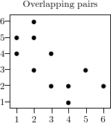
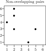
As you can see, the fact that large and small numbers alternate causes a significant deviation from the equidistribution of the points.
For a number of generators it is possible to derive analytical bounds for the deviation from the equidistribution of s-dimensional tuples as measured by the discrepancy.
If one does not restrict oneself to form tuples out of consecutive numbers, the resulting test will be able to find more subtle kinds of correlations without resorting to high dimensions s. While this modification hardly changes the empirical testing, only in the case of the EICG analytical bounds have been derived for this generalized serial test.
Now that we have clarified the intuitive understanding of the concept of testing pseudorandom sequences, we will turn to the mathematical treatment of the subject. Rather than providing a full scale discussion of the mathematical objects and formalisms involved, which would exceed the scope of this thesis, we want to present an introduction targeted at the mathematical layman. Our aim in this section is to introduce as much of relevant concepts as is necessary to be able to explain the problems one faces when testing pseudorandom numbers and comparing PRNG. We refer to [85] for an in-depth discussion.
There is more than one mathematical approach to this topic. The following list tries to introduce the different viewpoints and gives references for further reading.
In our context, this branch of mathematics focuses on the equidistribution of a sequence of numbers.
Various measures for the quality of the equidistribution were developed over the years, of all these numbers, the discrepancy is the most common.
Theorems on the equidistribution usually deal with infinite sequences, thus they are not particularly useful in conjecture with finite (or periodic) sequences. For example, equidistribution of a sequence can be defined in terms of the discrepancy in the following way:

This approach targets the complexity and information content of the sequence in question. One of the possible measurements is the minimal size of a computer a program (or a Turing machine) which can reproduce the sequence. In the optimal case, the program code will have to explicitly contain the sequence in order to print it. Any possible shortcuts the program can use (like exploiting dependencies) will be a measure for the lack of randomness of the sequence.
Since all our sequences are generated by short programs, they a-priori fail this test. Thus we will not consider this notion in our tests.
A similar approach is to focus on the amount of information contained in the sequence. If the entropy is high enough, we will accept the sequence as a good approximation of random numbers. Another way to express this notion is to state that the sequence is not compressible.
Testing whether a sequence is compressible is not easy since all common implementations cannot achieve the theoretically possible compression. Only really bad PRN can be eliminated with programs like gzip or compress. Extending the capabilities of these programs (for example enlarging the range of the pattern search in gzip) might be a way to get a workable test. As far as we know, nobody has tried this yet.
For larger sequences, the distinction between these ideas start to blur, as the size of the information needed to transform one representation into the other becomes irrelevant.
A sequence of PRN can be used to construct a stream cipher. If “true random” numbers are used, this cipher is called the one-time pad and is provably secure. So it is natural to ask what properties the PRN must have to achieve a good level of security.
According to Rueppel [76] there are several approaches to the construction of a secure stream cipher: The information-theoretic approach considers the possibility in principle to derive the seed (i.e. the key) from an observation of the PRN, the system-theoretic approach tries to make breaking the cipher at least as hard as solving known “hard” problems like factoring or the discrete logarithm. The complexity-theoretic approach tries to make sure that the amount of work needed to break the cipher is of non-polynomial complexity, randomized stream ciphers increase the magnitude of the code-breaker’s problem by utilizing a public pool of random numbers.
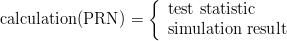
The basic idea of statistical testing can be summarized as follows: From a sample of supposedly random numbers a function called test statistic is calculated. As the distribution of this function is known for the case of real random numbers (otherwise the test does not make sense), one can determine which kind of results are extremely unlikely to occur. Typically this is formulated as intervals in the domain of the test statistic. These intervals (usually called critical region) are selected in a way that the probability that real random numbers lead to a test statistic there is smaller than the level of significance (usually 0.05, 0.01 or 0.005). If now for a sample of PRNG the test statistic falls into the critical region the common inference is to reject the sample.
All common tests rely on the idea of statistical testing. In the following we will try to elaborate on the motivation behind these tests, their mathematical foundation, their power and limitations, and how to interpret their results.
First of all, let us take a closer look at what we want to simulate. Our target are sequences of random numbers, which are realisations of a sequence of independent, uniformly distributed random variables.
Random variables (RVs) are one of the main building blocks in probability theory. They are used to assign each possible outcome (or, to be more exact, each reasonable set of outcomes) of an experiment a real number which is interpreted as the probability of this outcome.
But strictly speaking, the mathematical concept of RVs does not explicitly reflect our intuitive ideas about randomness of events, on the contrary: RVs are just simple, ordinary functions. One is tempted to ascribe mythical powers to RVs, like the ability to randomly select one of a set of possible events. This is not true, they only describe certain aspects of an idealized system which flips the metaphorical coin.
So where is the link between the mathematical world of RVs and the real life world of roulette tables ? Unfortunately there is none for single events. Even if a RV does in fact model a real world event, hardly any conclusions can be made about the outcome of the next single event. Even such unlikely events as winning the jackpot in a lottery do happen every now and then, and most people are not deterred by the extremely bad odds from playing every week. On the other hand some people are scared of travelling by plane because the probability of a safe flight is marginally less than one. In both cases our experience tells us that the probability alone cannot predict the next outcome.
But even such pretty definite sounding statements like “this event will occur with probability 1” cannot guarantee the outcome of an event. More insight into measure theory will tell us why such strange things can happen. For example, the probability that the next realisation of an U([0, 1[)-distributed random variable will be a rational number is zero. This does not stop the real world from delivering one of the infinite number of rational numbers, thus rendering the statement “This experiment will only return irrational numbers” incorrect.
We have seen that a RV cannot make concrete statements about a single outcome, so we might ask what statements about outcomes it can make at all. One way to formulate the meaning of probability is the following: [85, p. 10]
The probability assigned to an event expresses the expected average rate of occurrences of the event in an unlinked sequence of experiments.
We need to elaborate on two aspects of this definition as they are not as strict and unambiguous as commonly demanded from a good definition.
First, what do we mean by “expected” ? That seems to indicate that probability cannot be an intrinsic property on an event. There is no mathematically satisfying way to assign a probability to an event based on a (finite3) set of measurements, as it is extremely unlikely that another set of experiments will result in the same value. The common way out is to make assumptions about some parts of the experiment, like the Laplace assumption which assigns the same probability to all underlying events. These assumptions are based on a mental model of that event which includes a theory on how often something should occur. It is the mathematician, the physicist or just some observer who forms a mental model based on experiences or consideration. Such simplifying mental models of the real world are ubiquitous as they provide an essential simplification in the way we view the world. Other such simplifications include the concept of rigid bodies, fluids, or gases which are abstractions of “a bunch of molecules tied together by various forces”. Just as the laws of leverage rely in their formulation on the concept of forces and of rigid bodies the laws of chance depend on the concept of probability assigned to events.
The other critical word in the above definition is “unlinked”. By unliked we mean that the outcome of one experiment does not influence the outcome of any subsequent experiment. Common examples for unlinked experiments include drawing balls from an urn (with putting them back in !), casting a dice, or the roulette wheel. Please note that in all these examples there is a connection between two successive experiments as the first one does influences the second. It is a conscious decision by the observer that the re-shuffling of the balls in the urn caused by the first experiment does not affect the probability in the second one. This sounds almost like a paradox, as the re-shuffling surely does effect the outcome. But remember, just above we noted that the probability of an event does not determine the next outcome at all, so there is not contradiction here.
We have to be careful with sequences of PRN and their relation to independent random variables, too. The concept of independence is based on the concept of distributions. As we cannot ascribe distributions to numbers, we cannot use the term “independence” for sequences of PRN. We will use the word correlations to refer to any unwanted relationship between elements in the sequence.
As described above, the theory of random variables and probability tries to model aspects of the physical world. The fundamental principles of science demand justification in form of experiments for all such theories. For typical physical models such experiments are usually easy to set up and follow the same scheme of comparing an expected (calculated) result to the measurements of the actual physical event. If they differ more than inaccuracies in the measurements would allow, the theory is proven to be wrong. Philosophy of Science tells us that it is impossible to positively prove a theory.
Do the same principles hold for conjectures in the field of probability, too ? Unfortunately, they do not. Let us illustrate this with an example:
As a theory to test we might take the assumption that a given coin is fair, meaning that the probability it lands with the heads side up is 1∕2. How might an experiment designed to test this hypothesis look like ? Surely it will involve throwing the coin a number of times and then comparing the result to the prediction. Calculating the prediction based on the theory is simple, unfortunately the prediction assigns each possible outcome a positive probability. Thus regardless of the behaviour of the coin the result is consistent with the theory, as we cannot rule out the measured result. If we have no way to reject a theory, we have to find a different set of criteria according to which we can justify theories.
The common way out is statistical testing. It should be clear that statistical testing can never be as strict as testing in other areas. It is a heuristic approach to the problem. As such, it relies on the good judgement of the tester and is not objective. But before we elaborate on the shortcomings of statistical testing let us summarize the basic procedure again, already using the test for randomness as the example.
The alternative hypothesis H1 states that H0 is not true.
C∣H0) ≤ α.
This is the basic outline of all common empirical tests. We will discuss a few tests and their results later in this thesis. So what are the weak spots in this method of testing pseudorandom numbers ?
First of all, when testing sequences of numbers generated by a PRNG basic premises of statistical testing are violated.
The theory behind statistical testing assumes that we actually deal with random events. It is thus a circular argument to conclude from the result of such a test that the numbers in question are “random”. Only their statistical properties that are subject to the test, not the basic premise that the concept of random variables is a valid model for that experiment.
It is therefore not correct to speak of “statistical testing” with respect to PRN testing. A more appropriate term is “numerical testing” as the test examines only a numerical property of a fixed set of numbers.
The only “statistical” part of the test is the calculation what numerical values for the test statistic are considered to be good and which are considered to be bad.
The test statistic determines which aspect of the numbers we want to test.
Dividing [0, 1[ into the intervals  for 0 ≤ i < n, counting the hits in
each interval, and then calculating the χ2 statistic is a straight-forward test
statistic which aims the the overall equidistribution of the pseudorandom
numbers in [0, 1[. The choice of the bins (in this case intervals) seems to be
a natural one.
for 0 ≤ i < n, counting the hits in
each interval, and then calculating the χ2 statistic is a straight-forward test
statistic which aims the the overall equidistribution of the pseudorandom
numbers in [0, 1[. The choice of the bins (in this case intervals) seems to be
a natural one.
But what bins should we use to measure the finer aspects of
equidistribution ? We could use just a large value for n and keep the
intervals, but that would cause a problem with the validity of the χ2
approximation as the number of hits per bins decreases. An other option is
to use something like this: Define bin i as {x [0, 1[: ⌊x⋅k⌋≡ i (mod n)}
for some suitable values for k and n. Then the bins are no longer simple
intervals, but sets of intervals that are spread over the unity interval. The
value for k determines the width of each component interval.
Is there a natural choice for k ? We do not think so. But the choice can be important as the result of the test depends on it. Consider for example the set of numbers defined by {i∕m∣0 ≤ i < m} which is perfectly equidistributed in[0, 1[. For certain relations between k, n and m, like k∣m⋅n, the test will result in extremely bad χ2 statistics. As an example, consider the case k = n ⋅ m where all numbers i∕m fall into the same bin. For other values of k, this set of PRN will exhibit no weakness in this test.
We have seen that even such simple changes to the test statistic, like modifying the width of stripes, can completely change the result of the test. One can imagine that completely different layouts of bins will lead to a great variance in the test results, too. Thus we have to keep in mind that the choice of the test statistic, and thus to some extent the result of the test, is arbitrary.
One consequence of this fact is that we cannot declare one sequence of PRN to be better than a second one just because we found a test where the first one rates better, as a slightly modified test might produce exactly the opposite result.
What we strive for are numbers who behave in most respects like realisations of U([0, 1[)-distributed RVs, so it is a natural question how such ideal random numbers will perform in our statistical test. The answer to this is quite simple: If we conduct a test at the significance level α then a sequence of random numbers will fail the test with probability α. If we have set α = 0.01 then we can expect a failure about once every hundred tries.
As PRN should model all aspects of real random numbers, they should fail statistical tests at about the same rate.4
It is therefore not advisable to outright reject a sequence of PRN based on its failure in single tests.
Classic statistical tests examine if the test statistic does not deviate from its expected value too much. If we are only interested in the expected outcome of a similar simulation problem, such one-level statistical tests are all we need in order to be confident about the accuracy of the simulation.
On the other hand we might be interested in the distribution of the simulation’s outcome. For this goal hitting the expected value is not enough, the variance of the result is now important, too. Thus we will demand the same behaviour from the test statistic, too.
Let us illustrate this principle with an example. We want to test the well known strategy of doubling the ante in a game of roulette. It is supposed to guarantee winning the initial ante and works like this: If we do not win in the first round (and therefore win twice the ante) the ante is doubled for the next round. If this round is won, we get back four times the initial ante while we invested three times the initial ante resulting in a net win of one ante. In case of bad luck we double the ante again hoping for eight times the ante for an investment of seven. As we hope that we will finally win before our capital is drained a net win seems to be certain.
In order to simulate this we need random numbers to determine whether we will win the current bet. The probabilities are 18∕37 for winning and 19∕37 for losing each round, respectively. It seems to be natural to use the lengths of runs as a test statistic to test our source of PRN for its fitness to simulate a real roulette table. The probability that the maximal run length in 500 tries is greater than 15, is smaller than all usual values for α, so according to the corresponding statistical test we should reject all sequences where such runs do occur.5
When we now run the simulation with these prescreened sequences we will never ever experience a loss as long as we have enough money for 15 steps of doubling the ante. Thus we should conclude that the strategy works. As we know, this is not true. So what went wrong with our simulation ?
The statistical test considered it equally important whether the sequence in question was “well-behaved” or not, whereas the simulation assigned completely different weights to those cases. Thus the area that the test considered to be insignificant (smaller than α) played a major role in the simulation (more than 1∕2).
There are some other cases of simulations where we are not so much interested in the average case, but in the extreme ones. Consider for example all those safety measures in power plants or other machinery where a rare sequence of occurrences might lead to catastrophic results. When simulating these security systems one must not a priori exclude unusual sequences.
Please note that the distinction between level-1 and level-2 tests (tests which test the distribution of the results of a level-1 test) is arbitrary. The test statistic of a level-2 test is just another function of the underlying set of PRN, too.
One might be tempted to use a set of statistical test to once and for all declare one generator superior to another generator. Intuitively this makes sense, especially when comparing two generators of the same type. A common use for this heuristic is the selection of optimal parameters for the LCG based on its lattice structure [29, 73].
But is this judgement mathematically justified ? Leeb explains in [59] that such judgement is not justified as all possible sequences of PRN of a given finite length pass exactly the same number of statistical tests.
In order be able to use statistical tests as a criteria for the selection of PRNG the user has to declare which properties he considers important. With this knowledge it is possible to weight the tests and therefore select a suitable generator for this specific application.
Both statistical tests and simulations use a set of PRN to perform a more or less elaborate calculation.
In a statistical test we draw a conclusion from the right side to left: Based on the difference between expected and calculated value we judge the quality of the PRN.
A simulation operates the other way round. Based on the (hopefully) known quality of the PRN we hope that the simulation result is correct.
While generic statistical tests can be used for this reasoning, one can increase their value by designing the tests to closely model the simulation. Thus the tests can target exactly those properties in the PRN which will be significant in their application.
In order to conclude this chapter on the notion of randomness let us recapitulate what we know about testing a generator, and how we should proceed when we face the task of selecting a generator for a particular simulation problem.
Furthermore, analytical investigations can yield some insight in the overall structure of a generator’s output which can be compared to the properties required in the simulation. The lattice structure of the LCG might be actually useful in Quasi-Monte Carlo integration whereas it can be harmful in geometric problems, e.g. the nearest-pair test [14, 54].
In this chapter we will discuss analytically derived properties of the explicit inversive congruential generator (EICG). We will use results obtained for the LCG to serve as a reference as the LCG is the most commonly used generator. Let us start by repeating the definition of the EICG:
ℤp. The explicit inversive
congruential generator (abbreviated as “EICG”) with parameters p,a,b,
and n0 defines a sequence (yn)n≥0 in ℤp by
 | (3.1) |
Please remember that we perform all calculations except the final scaling in the finite
field ℤp = {0, 1, 2,…,p - 1}. ℤp* will denote the non-zero elements of ℤ
p, that is
ℤp* = {1, 2, 3,…,p - 1}. The over-line a denotes the multiplicative inversion in
ℤp for all non-zero elements a ℤp*. With the special case 0 = 0 added,
x x is a bijective function from ℤp onto ℤp. Furthermore, we have x = x
and x = xp-2 for all x ℤ
p. The latter identity is due to Fermat’s Little
Theorem.
x is a bijective function from ℤp onto ℤp. Furthermore, we have x = x
and x = xp-2 for all x ℤ
p. The latter identity is due to Fermat’s Little
Theorem.
Note that from the explicit definition of the sequence (yn)n≥0 we can easily derive a recursive description:
In order to achieve maximal period length p, the parameters a,b, and n0 can be freely chosen from ℤp as long as p is prime and a≠0. To see this, consider the function f(n) := a ⋅ (n0 + n) + b which is composed of bijective functions in ℤp and thus is bijective, too. As n + p = n in ℤp we have f(n + p) = f(p) for all n, thus the sequence (yn)n=0∞ is purely periodic with period length p.
We will only consider full period generators, that is a≠0.
We will write eicg(p,a,b,n0) to denote the output of a particular instance of the EICG method. Unlike Leeb [59, p. 89] we mean the whole infinite (but periodic) sequence, and not just the first p numbers. This way, no special treatment of wrap-arounds is needed when considering subsequences.
The choice of parameters is simple for an EICG, but not all choices will lead to completely different pseudorandom numbers. In this section we will examine the relations between EICGs with the same modulus, but different parameters a, b, and n0.
These results are helpful for the implementation, as one can eliminate an addition modulo p, as well as to the theoretical investigation as they provide a very elegant way to describe sub-streams. We will elaborate on this idea which is due to Niederreiter [71, p. 5] later on.
First of all, let us make a rather trivial observation on the role of the parameter n0.
Observation 3.1 Let (yn)n≥0 = eicg(p,a,b, 0). Then we can write the sequence eicg(p,a,b,n0) as (yn)n≥n0. In other words, the second sequence is first one shifted by n0.
Proof: This relation follows from the fact that n and n0 appear only as their sum n + n0 in the definition of the EICG. __
The following observation is taken from Leeb [59, p. 89]; it states that one of the parameters is redundant.
Proof: We base the proof on the recursive definition of the EICG. As the recursion does only depend on a, which is constant, it is sufficient to show that the y0 of these generators are equal. In the first two cases we have
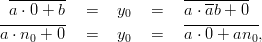

_
The third equality can be used to rewrite any EICG as an EICG with b = 0, but a different value for n0. Thus the generating formula can always be rewritten as

which saves one addition. The addition n0′ + n can be implemented by simply incrementing the previous value modulo p, thus we need to perform only one increment, one multiplication, one inversion, and one division to generate the next pseudorandom number.
There is an obvious connection between eicg(p,a,b,kn0) and eicg(p,ka,b,n0), too:1
Observation 3.3 Let p be prime, a,k ℤp*, and b ℤ
p.
The sequence eicg(p,ka,b,n0) can be obtained by selecting every k-th element
from the sequence eicg(p,a,b,kn0).
Proof: The sequence generated by taking every k-th element in the sequence eicg(p,a,b,kn0) = (yn)n≥0 can be written as (ykn)n≥0. We have
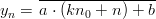
and thus
These three observations give us the tools to show that all maximal period EICGs can be derived from the “mother-EICG” eicg(p, 1, 0, 0) in the following way:
Can these insights help us in the theoretical investigation on how samples from an EICG behave under various tests ? Yes, they provide a very convenient and elegant formalism to describe subsequences and various kinds of s-tuples generated from the stream of pseudorandom numbers. With this formalism, the proofs of discrepancy estimates and non-linear properties are very concise.
First of all, we do not need to bother with the parameter n0 in the theoretical investigation as we can always rewrite the EICG to one with n0 = 0.
Second, any property of a sequence of EICG numbers, which is valid independently of the parameters used, is immediately valid for subsequences consisting of every k-th element. One direct consequence of this is, that once we can prove that pairs of consecutive numbers are uncorrelated for all valid parameters, we can rule out the possibility of long-range correlations at critical distances. See [10, 20] for a discussion of such problems inherent to the LCG.
The third gain, due to Niederreiter [71], is to be able to write almost arbitrary s-tuples formed out of the stream of EICG numbers as parallel streams. Such s-tuples as usually used to examine the correlation between successive numbers. For example, the overlapping serial test (see page §) tests the equidistribution of the vectors
 | (3.6) |
for n = 0, 1,…,p - 1 in order to test the PRN (yi)i≥0 for correlations. If we pick the first coordinate of each vector we get the original sequence. Picking always the second results in the original sequence shifted by one. According to the above equivalences we can write this shifted sequence as an EICG with the same parameter a, n0 = 0, and a different b. Thus we have
 | (3.7) |
where (yn(i)) n≥0 is the sequence generated by the EICG eicg(p,a,a(i- 1) + b, 0). The obvious generalisation is to allow almost arbitrary EICGs eicg(p,ai,bi, 0) for each coordinate.
In the following, we will prove all statements on the behaviour of s-tuples in terms of these parallel streams. For that, we will need to restrict the possible values for the ai and bi in order to avoid certain special cases like a1 = a2 ∧ b1 = b2. As we will see later in the various proofs, we need the condition aibi≠ajbj for all i≠j. Thus we have the following definition:
Definition 3.1 (Parallel Streams) Let p be prime, 1 ≤ s < p, and a1,…,as ℤp*,
b1,…,bs ℤp such that alb1,…,asbs ℤp are distinct. Then we put
 | (3.8) |
and define a sequence (yn)n≥0 in the s-dimensional affine space over ℤp by putting
An interesting special case of parallel streams, which is more general than the overlapping s-tuples considered above, can be obtained as follows. Choose an integer m ≥ 1 with gcd(m,p) = 1 and integers 0 ≤ n1 < n2 < … < ns < p and put

where the yn are as in (3.1). This sequence of points in ℤps can be written in terms of parallel streams according to Definition 3.1 by putting ai = am and bi = ani + b for 1 ≤ i ≤ s. It is easy to show that the aibi are distinct, thus all results concerning parallel streams are valid for this general method of composing s-tuples, too.
The non-overlapping tuples yn := (ysn,ysn+1,…,ysn+s-1) are covered by the concept of parallel streams, too. To see this, set ai = sa and bi = a(i - 1) + b for i = 1,…,s.
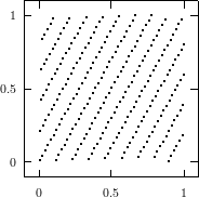
The best known structural property of any pseudorandom number generator is the lattice structure of the LCG. Coveyou/MacPherson [9] and Marsaglia [65] noted first that s-tuples formed from successive LCG-numbers form a lattice in the s-dimensional cube. Figure 3.1 depicts the lattice formed by plotting overlapping 2-tuples for the full period of two “toy” generators. “Production quality” generators exhibit the same structure, you just have to zoom into the image to see the pattern.
The shape of the lattice depends very strongly on the parameters a and b of the LCG. Thus various measurements on the coarseness of the lattice are used to select suitable parameters a and b. That way, a weakness of the LCG turns into a strength, as one can guarantee a well-behaved lattice for low dimensions as long as the parameters are chosen well enough.
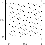
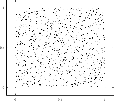
Does the EICG exhibit a similar structure ? Figure 3.2 suggests that the EICG does not possess this linear property, although one can see some other regularities. In fact, one can prove a very stringent non-linearity property for s-tuples taken from an EICG. The theorem describing this is due to Niederreiter [71].
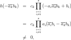
Theorem 3.1 Let yn =  as in Definition 3.1, then every
hyperplane in ℤps contains at most s of the points y
n, n = 0, 1,…,p - 1, with
yn(1)
as in Definition 3.1, then every
hyperplane in ℤps contains at most s of the points y
n, n = 0, 1,…,p - 1, with
yn(1) y
n(s)≠0. If the hyperplane passes through the origin of ℤ
ps, then it contains
at most s - 1 of these points yn.
y
n(s)≠0. If the hyperplane passes through the origin of ℤ
ps, then it contains
at most s - 1 of these points yn.
Proof: All calculations in this proof are performed in the finite field ℤp. Furthermore, remember that according to Definition 3.1, the aibi are distinct.
A hyperplane Hc,c0 in Zps is uniquely defined by a vector c = (c
1,…,cs) ℤps \{0}
and a scalar c0 ℤp as Hc,c0 = {x Zps | x ⋅ c = c
0}. We restrict our search for points
on a hyperplane n W := ℤp \{-a1b1,…,-asbs}. Thus for n W we have according
to (3.8) yn(1),…,y
n(s)≠0, therefore we can rewrite the hyperplane equation for y
n
as
By clearing denominators, we see that n is a root of the polynomial
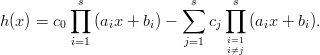
If c0≠0, then h is a nonzero2
polynomial of degree s over ℤp. Since such a polynomial has at most s roots in ℤp, the
hyperplane Hc,c0 contains at most s of the yn with n {0, 1,…,p- 1}\{-a1b1,…,-asbs}.
If c0 = 0, that is 0 Hc,c0, we get
whose degree is at most s - 1. It remains to show that h is not the zero polynomial. As c is not the zero vector, one of its coordinates is nonzero. For ck≠0 we have
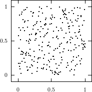
This theorem proves that s-tuples taken from an EICG do not form any linear structure such as a lattice. But that does not mean that no other kind of pattern emerges in plots of pairs of consecutive3 numbers. For example, consider Figure 3.3, where one can see a hyperbola-like structure in the upper left and lower right corner. Eichenauer-Herrmann and Wegenkittl are currently preparing a paper discussing these properties of the EICG.
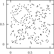
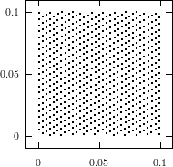
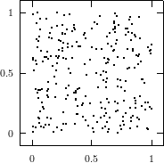
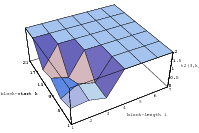
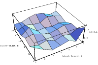
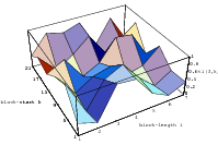
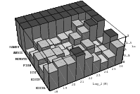
All the plots so far contained all the overlapping pairs available from the full period of the generator. This way, the underlying structure of the generator is perfectly visible. But usually one does not utilize the full period of any generator; a common rule of thumb is to use not more than the square root of the period. Thus the LCG will never be able to build up the full lattice and the EICG will contain only a few points on hyperbola. Figure 3.4 depicts the lattice of lcg(65536,325,1,1), the first image shows the full lattice in a zoomed view, the second one contains only 256 points, which corresponds to the square root of all possible points.
These figures clearly demonstrate that any regularities a generator develops over the full period are not necessarily present when only a fraction of the available numbers is used. The recommendation never to exhaust the full period can be further justified by the following argument: The PRNG is supposed to simulates drawing numbers from an urn with putting the numbers back into the urn, but in fact the typical PRNG empties the imaginary urn before it puts all numbers back when the period is exhausted. The difference between “drawing with replacement” and “drawing without replacement” is small as long as only a fraction of all numbers are drawn from the urn.
The discrepancy is a widely used and well studied measure for the equidistribution of a set of points. In this section we will try to give a motivated definition, some theoretical background, and summarize all published results concerning the EICG.
There are at least three approaches to the notion of discrepancy, one stems from statistics, one from geometric reasoning, and one from numerical integration. We will use the latter. An extensive introduction to discrepancy can be found in Niederreiter [70, Chapter 2].
We will use the following setting: The closed s-dimensional unit cube  s
= [0, 1]s
will be the integration domain in which we will try to integrate the function f by using
the quasi-Monte Carlo integration
s
= [0, 1]s
will be the integration domain in which we will try to integrate the function f by using
the quasi-Monte Carlo integration
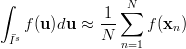 | (3.9) |
with x1,…,xN  s
. Ideally, we hope that the approximation converges to the integral
as the number of points increases. If this is the case for a reasonable class of functions,
say, for all continuous f on
s
. Ideally, we hope that the approximation converges to the integral
as the number of points increases. If this is the case for a reasonable class of functions,
say, for all continuous f on  s
, then we call the (infinite) sequence (x1,x2,…) uniformly
distributed in
s
, then we call the (infinite) sequence (x1,x2,…) uniformly
distributed in  s
. One can show that this definition of “uniformly distributed” is quite
independent of the class of functions; using the Riemann-integrable functions yields
the same test as using the characteristic functions of a very simple set of
intervals.
s
. One can show that this definition of “uniformly distributed” is quite
independent of the class of functions; using the Riemann-integrable functions yields
the same test as using the characteristic functions of a very simple set of
intervals.
Whereas the limit of the integration error can be used as a qualitative measure for the distribution properties of an (infinite) sequence of points, one can use the integration error in the finite case as a quantitative measurement of the equidistribution of the finite sequence (xn)n=1N.
In order to get a workable measurement, we have to state which family of functions f we consider for the integration, and how we condense all the integration-errors for each function from the family into one single number.
The general concept of discrepancy uses the set of characteristic functions of axis-parallel cubes in Is := [0, 1[s as the functions to integrate and the supremum as the condensing function. Formally, we can write this in the following way:
If Ω = (xn)n=1N is a finite sequence in Is, and B an arbitrary subset of Is, then we can express the quasi-Monte Carlo integration of the characteristic function4 cB in terms of the number of xi in B,

as
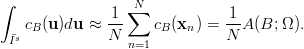
Based on this, the error when integrating cB can be written as 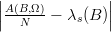 , where λs(B) is the
s-dimensional volume5
of B. Thus we can write the general notion of the discrepancy of a finite sequence Ω of points in
Is for an arbitrary6
family
, where λs(B) is the
s-dimensional volume5
of B. Thus we can write the general notion of the discrepancy of a finite sequence Ω of points in
Is for an arbitrary6
family  of sets as
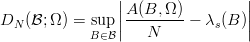 | (3.10) |
From this general definition we can derive the definition of the two most important incarnations of discrepancy as follows:
Definition 3.2 The star discrepancy DN*(Ω) = D
N*(x
1,…xN) of the finite
sequence Ω is defined by DN*(Ω) := D
N( *; Ω), where * is the family of all
subintervals of Is of the form ∏
i=1s[0,u
i[.
*; Ω), where * is the family of all
subintervals of Is of the form ∏
i=1s[0,u
i[.
Definition 3.3 The (extreme) discrepancy DN(Ω) = DN(x1,…xN) of the
finite sequence Ω is defined by DN(Ω) := DN( ; Ω), where is the family of all
subintervals of Is of the form ∏
i=1s[u
i,vi[.
While DN and DN* are the classical figures for measuring the equidistribution, they are far from being the only ones. Interesting variations of the basic idea are the isotropic discrepancy, which uses the family of convex sets instead of axis-parallel cubes, or the L2-discrepancy, which uses the 2-norm instead of the supremum. Especially the L2-discrepancy has received a lot of attention recently as it is suitable for empirical testing [38] and has a number of interesting theoretical properties [80, 62]. Another measurement worth mentioning is the weighted spectral test [40, 46, 44, 41, 47].
Let us quickly state a few general results concerning discrepancy. They will help us to interpret the main results of this chapter. We once again refer to Niederreiter [70, p. 14ff, p. 166ff] for proofs and further references.
Proposition 3.1 For all finite sequences Ω consisting of N points in  s
we have
s
we have

and

In dimension one, that is s = 1, it is possible to express the discrepancy as a relatively simple formula operating on the ordered list of points.
Proposition 3.2 If 0 ≤ x1 ≤ x2 ≤… ≤ xN ≤ 1, then
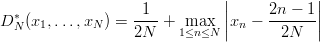
and

From these formulae, as well as the well known fact that sorting is of complexity
 (N log N), it is easy to see that one can calculate the discrepancy in the
one-dimensional case in (N log N) + (N) steps. Using a memory versus speed
tradeoff [34] it is possible to get the complexity down to (N). In higher
dimensions s calculating the discrepancy is of complexity (Ns), making
any reasonable empirical testing computationally infeasible. Probabilistic
algorithms [89] can be employed to calculate tight upper bounds for a given
Ω.
(N log N), it is easy to see that one can calculate the discrepancy in the
one-dimensional case in (N log N) + (N) steps. Using a memory versus speed
tradeoff [34] it is possible to get the complexity down to (N). In higher
dimensions s calculating the discrepancy is of complexity (Ns), making
any reasonable empirical testing computationally infeasible. Probabilistic
algorithms [89] can be employed to calculate tight upper bounds for a given
Ω.
What do we know about the behaviour of DN with increasing N ? If the sequence
of point is indeed uniformly distributed in  s
, then we know that lim N→∞DN = 0. For
a sequence of uniformly distributed random points we know that lim N→∞DN = 0 with
probability one. But in order to use the discrepancy as a figure of merit for
finite sequences, we need to know exactly how DN converges for random
sequences. Luckily, the following result (due to Kiefer [49]) provides us with the
benchmark according to which we can judge the discrepancy bounds derived for
PRN.
s
, then we know that lim N→∞DN = 0. For
a sequence of uniformly distributed random points we know that lim N→∞DN = 0 with
probability one. But in order to use the discrepancy as a figure of merit for
finite sequences, we need to know exactly how DN converges for random
sequences. Luckily, the following result (due to Kiefer [49]) provides us with the
benchmark according to which we can judge the discrepancy bounds derived for
PRN.
Proposition 3.3 (Law of the iterated logarithm) Let z1,z2,z3,… be a
sequences of uniformly distributed random points in  s
, then we have
s
, then we have
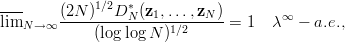
where λ∞ is the Lebesgue measure on the space of all infinite sequences in  s.
s.
The discrepancy is per definition an upper bound for the quasi-Monte Carlo integration error for a very limited class of functions, namely the characteristic functions of axis-parallel cubes. A classic result by Hlawka uses the discrepancy to derive an error-bound for a large class of functions.
Proposition 3.4 (Koksma-Hlawka inequality [70]) If f has bounded
variation V (f) on  s
in the sense of Hardy and Krause, then for any x1,…,xN
Is we have
s
in the sense of Hardy and Krause, then for any x1,…,xN
Is we have
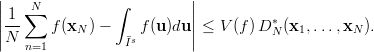
Why is this inequality so important ? For the Monte Carlo numerical integration, which is based on “random numbers”, one cannot derive an a-priori7 error bound on the integration error. It is only possible to state a probabilistic error bound, a shortcoming that is often not acceptable. The inequality of Koksma-Hlawka on the other hand, is a hard bound on the integration error. Thus in order to get such a bound for the Monte Carlo method, one has to calculate the discrepancy for the numbers used, which is not feasible in practice. The way out is to use a set of numbers for which bounds on the discrepancy are known in advance, such as (t,m,s)-nets or PRNGs for which such bounds are available.
On the other hand, if we want our PRNG to model a U[0, 1[ distributed random
variable as closely as possible, the law of the iterated logarithm provides us with
the correct order of magnitude for the discrepancy. One can argue that any
results concerning the discrepancy of a particular generator which shows a
rate of growth close to (N-1∕2 log log N) is a sign for the right amount of
“randomness” in the generator. Empirical evidence seems to support this
argument. In any case, the discrepancy is certainly the most widely used
figure of merit in theoretical analysis of pseudorandom number generation
algorithms.
In order to prove discrepancy bounds, we need a variety of auxiliary results. Unfortunately it is not possible to include the proofs for these lemmata without exceeding the scope of this thesis, as well as alienating the target audience. Thus we will only list the results and give references to the proofs.
The basic approach to derive discrepancy bounds for PRNG is due to Niederreiter [70], who established a link between the discrepancy of a finite sequence of points with rational coordinates and certain exponential sums. As most common PRNG use integer arithmetic combined with a final scaling operation, this approach is perfectly suited for the study of the output of such generators.
Niederreiter’s proof [70, §3.2] is elementary, although rather tricky. Hellekalek [39] gave a proof based on dyadic harmonic analysis. A detailed proof can be found in Weingartner [87].
In correspondence with the literature [71, 70], we will use the following definitions:
For a prime p ≥ 5 let Cs*(p) be the set of all nonzero h = (h
1,…,hs) ℤs
with |hi| < p∕2 for 1 ≤ i ≤ s. For such h, put r(h,p) = ∏
i=1sr(h
i,p) with
r(h,p) = p sin(π|h|∕p) for h nonzero and r(0,p) = 1. Furthermore, set
χ(n) = e2π n∕p for n Z
p, and let u ⋅ v denote the standard inner product of
u,v
n∕p for n Z
p, and let u ⋅ v denote the standard inner product of
u,v  s.
s.
Although some of the Lemmata below do not need this restriction, we will consider only the case of prime moduli here.
Lemma 3.1 For a prime p ≥ 2 and y0,y1,…,yN-1 ℤps, let Ω be the finite
sequence (xn = yn∕p)n=0N-1. Then
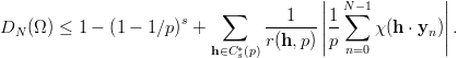
The following Lemma is due to Niederreiter [71, Lemma 2] which improves [70, Corollary 3.11].
Lemma 3.2 Let p ≥ 5 be a prime and let y0,y1,…,yN-1 ℤps. Suppose the
real number B is such that
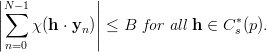
Then the discrepancy DN of the finite sequence (xn = yn∕p)n=0N-1 satisfies
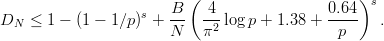
In order to derive the bound B for the EICG we need the following two Lemmata, the first one is due to Cochrane [7], the second is a variant of the Bomberi-Weil bound for exponential sums (see Moreno and Moreno [68, Theorem 2]):
Lemma 3.4 Let Q∕R be a rational function over ℤp which is not of the form
Ap - A with A ℤ
p(x). Let s be the number of distinct roots of the polynomial
R in ℤp. Then we have
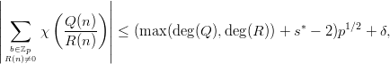
where s* = s and δ = 1 if deg(Q) ≤ deg(R), and s* = s+1 and δ = 0 otherwise.
The Koksma-Hlawka inequality can be used to derive a lower bound on the discrepancy of a finite sequence of points. All that is needed is a function with a known integral and bounded variation. In light of the previous lemmata it seems natural to use a function for which the Monte Carlo integration can be expressed in terms of exponential sums. The following result is due to Niederreiter [70, Cor. 3.17].
Lemma 3.5 For a prime p ≥ 2 and y0,y1,…,yN-1 ℤps, let Ω be the finite
sequence (xn = yn∕p)n=0N-1. Then, for any nonzero h ℤs, we have
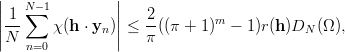
where m is the number of nonzero coordinates of h.
Unfortunately, we cannot prove a lower bound on the generic sum ∑ χ(h ⋅ yn) for finite sequences of points generated by an EICG. But we are able to prove such bounds for a slightly different exponential sum EN(χ; d,e), which we can link to sequences generated by an EICG, and which is a special case of the sum in Lemma 3.5. This approach is due to Eichenauer-Herrmann and Niederreiter [23]. All lemmata and theorems concerning lower bounds are taken from this paper.
For d = (d1,…,ds) ℤps and e = (e
1,…,es) ℤps we define
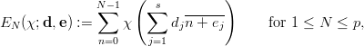 | (3.11) |
and put E(χ; d,e) := Ep(χ; d,e).
See [23] (Theorem 1 and Corollary 1) for the proofs, which are similar to the proofs of Theorems 3.2 and 3.3. Besides these upper bounds, we know the average value of the EN(χ; d,e), according to the next Lemma.
Proof: We set dj,m,n := dj(n + ej -m + ej). With e = (e1,…,es) we get
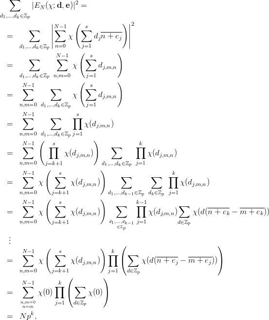
 ℤpχ(d ⋅ k) = 0 for k Zp,k≠0 and p otherwise. __
Applying Lemma 3.5 on a finite sequence of points generated by parallel streams of
EICG according to Definition 3.1, and h = (1, 1, 0,…, 0) ℤs we get for s ≥ 2
ℤp2 and e = (b
1a1,b2a2) ℤp2. Similarly, for h = (1, 0,…, 0) ℤs
and s ≥ 1 we have
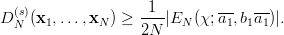 | (3.13) |
We now have the tools necessary to derive upper and lower bounds on the discrepancy of finite sequences of points generated by parallel streams of EICG numbers. But as a reference, let us first look at the result available for the LCG, which will once again serve as a reference.
According to [70, Theorem 7.4] we have for the multiplicative linear congruential generator the following statement: For s ≥ 2 and for an average multiplier a, the discrepancy of the finite sequence of s-dimensional points consisting of all M - 1 overlapping tuples from lcg(M,a, 0, 1) obeys

where the implied constant depends only on s.
We first turn our attention to upper bounds; we will prove both bounds for the full, as well as or parts of the period. These bounds are relevant in two ways:
Please note that the following theorems do not depend on the choice of any parameters; they are valid for every single full period EICG. This is in sharp contrast to the bounds known for the LCG, which is only deals with the average over all multipliers, and thus tells us nothing about a particular generator. Furthermore, in the case of the LCG no bounds are known for parts of the period in dimensions s ≥ 2.
As one can guess from the lemmata listed above, the proofs involve exponential sums which need to be rearranged in a way to be able to use Lemma 3.4.
The following two theorems are due to Niederreiter [71].
Theorem 3.2 For p ≥ 5, prime, and 2 ≤ s < p set xn = yn∕p based on the yn of Definition 3.1. Then we have for the discrepancy of the finite sequence (xn)n=0p-1 the following upper bound:

Proof: For h = (h1,…,hs) Cs*(p) put
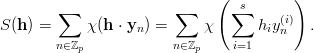
We now restrict the sum to those terms where yn(i)≠0 by using the same set W as in the proof of Theorem 3.1 as the summation domain. By noting that card(ℤp \W) = s and using the triangle inequation we get
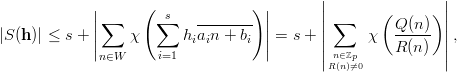
where Q∕R is the rational function over ℤp given by
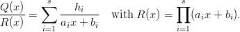 | (3.14) |
As all ai are nonzero, we have deg(R) = s < p. Furthermore, as at least one of
the hi is nonzero, the uniqueness of the partial fraction decomposition for
rational functions implies that Q≠0 and deg(Q) < s = deg(R). In order to
apply Lemma 3.4, we have to show that Q∕R is not of the form Ap - A with
A ℤp(x), where ℤp denotes the algebraic closure of the field ℤp, and ℤp(x)
denotes the field of rational functions over ℤp. If this were the case, we would
have
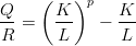
with polynomials K,L over ℤp and gcd(K,L) = 1, and thus
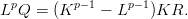 | (3.15) |
Since we have demanded gcd(K,L) = 1, L cannot divide K or (Kp-1 -Lp-1), thus Lp must divide R. As deg(R) = s < p, that can only be the case if L is a nonzero constant polynomial which implies deg(Lp) = 1. Comparing the degrees in (3.15) yields deg(Q) ≥ deg(R), which contradicts the degrees derived from (3.14). Thus we can apply Lemma 3.4, and this leads to
 | (3.16) |
The rest follows from Lemma 3.2. __
Theorem 3.3 For p ≥ 5, prime, and 2 ≤ s < p let the finite sequence (xn = yn∕p)n=0p-1 be like in Theorem 3.2. Then we have for the discrepancy of the first N points the following upper bound:
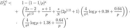
Proof: Just as in the proof of Theorem 3.2 we need to derive a bound for an exponential sum to be able to apply Lemma 3.2. This time the summation domain is not ℤp, thus we need to rewrite the sum in a rather tricky way.
For h = (h1,…,hs) Cs*(p) put
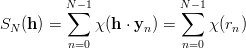
with rn = ∑
i=1sh
iyn(i) for n ≥ 0. We can now rewrite S
N(h) using the fact that
∑
uℤpχ(uk) evaluates to 0 for k≠0 and to p otherwise.
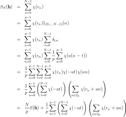
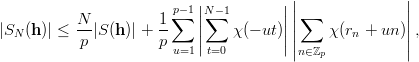 | (3.17) |
and examine each of the terms on the right side.
We want to apply Lemma 3.4 on the rightmost term: For 1 ≤ u ≤ p- 1 we have, by the same argument as following (3.14)
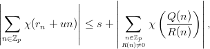
where Q∕R is the rational function over ℤp given by
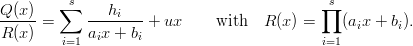
Once again, we claim that Q∕R is not of the form Ap - A with a rational
function A ℤp(x). From the definition of R and Q we have deg(R) = s
and deg(Q) = s + 1, as all the neither the ai nor u can be zero. For if we
had
with polynomials K,L over ℤp and gcd(K,L) = 1, then the argument following (3.15) shows that L is a nonzero constant polynomial. Thus we have
for suitable e1,e2 ℤp with e1,e2≠0. Comparing the degrees of the polynomials in
this equation we get deg(e1Kp + e
2K) = 1, which implies deg(K) ≥ 1, hence
deg(e1Kp + e
2K) = p deg(K) > 1. This contradiction proves that we can apply Lemma
3.4, yielding
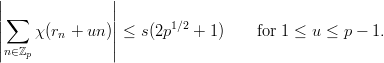 | (3.18) |
Furthermore, by rewriting the sum over t using some elementary equivalences like
χ(x) - 1 = e2π x - 1 = eπ
 x ⋅ (eπ
 x - e-π
 x) = eπ
 x ⋅ 2
x ⋅ 2 sin πx, we get
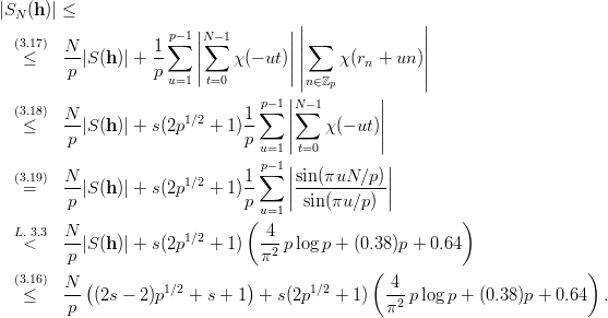 Cs*(p), and thus we can apply Lemma 3.2 to obtain the desired upper
bound on DN(s). __
Cs*(p), and thus we can apply Lemma 3.2 to obtain the desired upper
bound on DN(s). __
The theorems covering lower bounds are formulated in a different way. Instead of giving hard bounds for all EICG, these theorems state how many EICGs there must be exceeding a threshold value for the discrepancy. This kind of statement follows from the basic approach to the problem, namely combining upper bounds on exponential sums with their average values.
Lower bounds guarantee that the PRN are not perfectly equidistributed, they contain the irregularities found in “random” numbers, too.
The following three theorems are due to Eichenauer-Herrmann and Niederreiter [23].
Theorem 3.4 Let a2 ℤp*,b
2 ℤp, and c ℤp \{b2a2} be fixed. Let
0 < t ≤ , and set
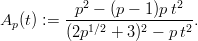
Then there exist more than Ap(t) values of a1 ℤp* such that for s-tuples from
the corresponding parallel stream of EICG numbers with b1 = a1c and s ≥ 2 we
have
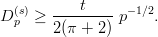
Proof: We rewrite the theorem in terms of EN by using (3.12). Thus we have
d = (d1,d2) = (a1,a2), and e = (e1,e2) = (b1a1,b2a2) ℤp2 with e
1≠e2, and we
need to show that there are more than Ap(t) values for d1 ℤp* such that
|E(χ; d,e)|≥ tp1∕2.
Now suppose there exist at most Ap(t) values of d1 ℤp* with |E(χ; d,e)|≥ tp1∕2,
i.e., there exist at least (p - 1) - Ap(t) values of d1 with |E(χ; d,e)| < tp1∕2.
From Lemma 3.6 (with s = 2) we know that |E(χ; d,e)|≤ 2p1∕2 + 3 for every
d1 ℤp*. Hence, observing that d
1 = 0 contributes nothing to the sum, we
obtain

which contradicts Lemma 3.7 (with s = 2, k = 1, and N = p). __
Theorem 3.5 Let a2 ℤp*,b
2 ℤp, c ℤp \{b2a2} and an integer N with
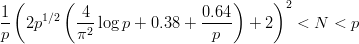
be fixed and set
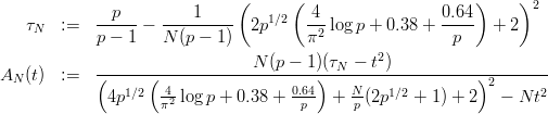
 . Then there exist more than AN(t) values of a1 ℤp* such that for
s-tuples from the corresponding parallel stream of EICG numbers with b1 = a1c and
s ≥ 2 we have
. Then there exist more than AN(t) values of a1 ℤp* such that for
s-tuples from the corresponding parallel stream of EICG numbers with b1 = a1c and
s ≥ 2 we have
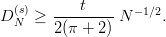
Proof: The proof is analogous to the last one. The only real difference is the handling of d1 = 0, where we need to apply Lemma 3.6 with s = 1. _
Using (3.13) instead of (3.12) we get a slightly different result. As the proof contains no new ideas, we omit it, too.
Theorem 3.6 Let c ℤp and 1 ≤ N < p be fixed. For real numbers t fulfilling
0 < t ≤ set
set
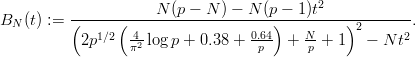
Then there exist more than BN(t) values of a1 ℤp* such that for s-tuples from
the corresponding parallel stream of EICG numbers with b1 = a1c and s ≥ 2 we
have
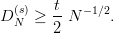
Restricting oneself to the ordinary serial test, i.e. is considering only overlapping s-tuples instead of vectors from parallel streams, it is possible to improve Theorem 3.6. See [23, Corr. 9] for details.
For congruential generators modulo a prime p, the following definition, due to Niederreiter [70], specifies another criteria which can be used to classify PRNGs.
Definition 3.4 For given s ≥ 1, a congruential generator producing the
sequence y0,y1,… ℤp passes the s-dimensional lattice test if the vectors
yn - y0,n = 1, 2,…, span the s-dimensional vector space ℤps, where

Theorem 3.7 An EICG with modulus p passes the s-dimensional lattice test exactly for all s ≤ p - 2. This is the optimal behaviour under this test.
Proof: As explained in 1.3.4, one can visualize any congruential generator modulo p with period length p as a permutation polynomial mapping n to yn. In the case of the EICG, this polynomial has degree d = p - 2 as we can write the the EICG formula as
according to the theorem of Euler-Fermat. The rest follows immediately from a theorem by Eichenauer, Grothe, and Lehn [13], which can also be found in Niederreiter [70, Theorem 8.2]. __
As explained is section 2.3.2, testing a pseudorandom number generator is a tricky task. Even if one decides which properties one wants to test for, designing the test itself involves a fair amount of statistic knowledge as to how the test should be parameterized as well as how the results should be judged.
In this chapter, we will try to give a survey of empirical tests concerning the EICG carried out by various authors. Since it will be inappropriate to spend too much time on discussing all design decisions in detail, we will only describe the motivation, the test procedure, and the results. For more information we refer to the original authors.
Another compilation of empirical test results concerning inversive generators can be found in [21].
The Digit Test, due to Leeb1 [58, 26, 61], tries to assess the distribution quality of a PRNG by looking at the g-adic representation of its output. If we only allow g = 2l, one digit in base g corresponds to l binary digits, which we can obtain by cutting out l consecutive bits in the computer representation of the numbers. This is a very efficient procedure which can be done by simple bitwise AND and shift operations. Let’s visualize this by an example, using 8 = 23 as the base and selecting the second digit which is corresponds to the three bits starting at position k = 4.
| Decimal | Binary | Base 8 | selected digit |
| 0.5859375 | 0.100 101 10 | 0.454 | 5 |
| 0.82421875 | 0.110 100 11 | 0.646 | 4 |
| 0.21484375 | 0.001 101 11 | 0.156 | 5 |
| 0.765625 | 0.110 001 00 | 0.610 | 1 |
| 0.16015625 | 0.001 010 01 | 0.122 | 2 |
| 0.48046875 | 0.011 110 11 | 0.366 | 6 |
Ideally, we expect the last column to be uniformly distributed over all possible digits. Furthermore, we can assume that if the original numbers are uncorrelated, this will hold for the sequence of digits, too. On the other hand, if we can prove that something is wrong with the digit sequence, this does not shed a good light on the original numbers.
What have we gained by mapping numbers to digits ? Basically this mapping plays the role of the “bins” discussed on page § and §. As discussed there, this mapping is used to make the problem manageable by drastically reducing the number of possible values for each number. Now we can easily count the occurrences of each different digit and perform correlation tests on them.
As a correlation test Leeb used the idea of the serial test (see p. §) with non-overlapping s-tuples. To measure the distribution of the s-tuples, a χ2 test was used; the resulting χ2-value was called t 1(s,k,l), the level-1 test statistic. This procedure was repeated 64 times, and all the χ2 values were compared to their expected distribution by a two-sided Kolmogorov-Smirnov test, yielding t2(s,k,l), the level-2 test statistic on which we will focus in the graphics.
Let’s summarize all the parameters which must be specified to turn the abstract idea of the Digit Test into a computer program.
{1, 2,…, 10}.
It should be clear by now that the hierarchical design of the complete testing procedure results in huge resource requirements both computationally as well as memory-wise to actually run the test. See Table 4.1 for the actual parameters used, and Table 4.2 for the generators tested. The computations were carried out using the pLab [57] PRNG testing framework, which is based on the author’s generator library.
|
| |||||||||||||||||||||||||||||||||||||||||||||||||||
|
| ||||||||||||||||||||||||||||||||||||||||||||||||||||||
For the graphics, the t1 value was transformed according to the expected χ2 distribution to yield a value which should be asymptotically equidistributed. Thus all points in the graphics on the left hand side should vary freely between 0 and 1. Values close to 0 signify a distribution of the s-tuples which is much to well-balanced, whereas values close to 1 indicate gross irregularities. The right hand graphics depict the KS-statistic t2, for which the critical region at the 1% level of significance is [1.63,∞). Any generator which features high values there (especially when reaching the cut-off point 2 in the graphics) fails in the test.
As Leeb in [58], we present here only a selection of the results, namely those for dimension s = 3. For each generator, the values of k and l were varied.
Interpretation: The digit test seems to be sensible to intrinsic properties of the LCG, as even the best one (FISH) fails the test for certain parameters. Leeb conjectures in [58] that the digit test is sensible on grid structures or long-range correlation as these are two features which are present in all LCG but are proven to be absent in inversive generators. Especially the lattice quality parameter 1∕νs seems to correlate with the digit test results. The better the lattice is (small values for 1∕νs), the higher the values for l and k must be to uncover deficiencies in the generator.
The overlapping serial test, first proposed by Marsaglia [66] as the “M-tuple test”, is in its basic setup quite similar to the digit test described above. The main difference is to use overlapping tuples. This modification is rather small in the implementation, but requires some statistical work to calculate the expected distribution as the tuples are no longer independent.
We will describe here the empirical tests done by Wegenkittl [85, 86, 61]. As the testing procedure was very similar to the digit test setup, we will only list the differences here. Whereas Leeb in the digit test used only one way to extract bits from the stream of pseudorandom numbers, Wegenkittl used two:
This time these blocks of bits were used to generate variable number of tuples. Whereas in the digit test the sample size M was always tuned to the subsequent χ2 test, Wegenkittl generated up to M = 226 tuples. From these tuples, a modified χ2 statistic t 1(o) was computed, resulting in the test-statistic χ o. Whereas the “normal χ2 test statistic” does not converge to a χ2 distribution for overlapping tuples due to the correlations, this modified one does (see [85, p. 57] for details). This procedure was repeated 32 times and the resulting empirical distribution of the χo values was compared to the theoretical one using a KS test.
The following graphics2 depict the results for all the generators used in the digit test, as well as for EICG7 which stands for eicg(231 - 1, 7, 0).
The left hand diagrams show the values for each of the 32 calculated t1(o) test
statistics as the lightness of each small rectangle. A white square signifies a low value
for t1(o), meaning perfect equidistribution of the tuples, whereas a black one signifies
extreme deviations. The transformation t1(o) lightness was chosen in such way that
each gray-scale level should be equally likely. Unfortunately, these diagrams are not
available for all parameters.
lightness was chosen in such way that
each gray-scale level should be equally likely. Unfortunately, these diagrams are not
available for all parameters.
In the right hand diagrams these 32 values were distilled into one single KS value representing the quality of their distribution. The critical region at the 1% level of significance is in this case [1.58,∞).
Interpretation:
Like the Digit Test, the overlapping serial test does uncover deficiencies in the
linear generators. Whereas the setup in the Digit Test focused on the number
of bits you can take from a number while still getting good distributions,
Wegenkittl turned his attention to the number of tuples one can generate before
the PRNG fails. The results are basically the same: even the best LCG has
a limited load-capability; if you start to do heady-duty computations using
many PRN you must be careful not to run into the breaking point of the
LCG. The traditionally rule of thumb concerning which percentage of the
period length one can safely use (up to  ) seems to be sound for the
LCG.
) seems to be sound for the
LCG.
The inversive generators are not perfect either, even they tend to fail the test at some point. But their load-capability is much better. Even when taking a high number of samples, their distribution quality decreases quite slowly.
A completely different kind of empirical test is the run test. The basic idea behind this test is to check if the occurrences of runs conforms to its expected value. There is a variety of different ways to implement this idea, but we will only describe the idea and Entacher’s implementation [24].
First of all, what do we mean by “runs” ? In a binary context, that is sequence consisting only of two symbols, a run is defined as a subsequence consisting only of one symbol. For example, consider the sequence

in which the brace indicate the runs.
As the common pseudorandom sequences are far from being binary, one has to transform them first. A straight forward way of doing this is
which is binary as xn+1≠xn for PRNG we consider. A run of 1s of length k corresponds to a monotonically increasing subsequence of length k + 1 in the original sequence called a “run up”. The distribution properties of these runs in a sequence of “really random numbers” is well known.
According to Wolfowitz [63] (see also Knuth [50, p. 68]) Entacher constructed an asymptotically χ2-distributed test statistic U r which involves counts for ascending runs up to length r. The calculation done by Entacher involved evaluating U6 100 times for each generator and testing this empirical distribution against the expected one using a KS test.
We will focus on Entacher’s results concerning the behaviour of LCGs and EICGs.
The list of generators tested include the previously defined generators FISH, ANSI,
MINSTD, and RANDU, as well as two other LCGs with a bad lattice structure:
LCG5 = lcg(231, 231 - 3, 0, 1) and LCG6 = lcg(231 - 1, 221 + 1, 0, 1). As examples for the
EICG Entacher used eicg(231 - 1,a, 0, 0) with parameter a {25, 210, 215, 220, 225, 230}
which he labeled EICG1 to EICG6.
The following figures3 depict the results; The sample size was varied between 212 and 224 (the labels are log 2(N)), the height of each square shows the resulting KS statistic. If the square is coloured dark gray, then the KS statistic exceeds the critical value for the significance level 0.01.
Interpretation: The run test seems to be able to distinguish good LCGs from bad ones. All basically randomly chosen EICG pass the test without any problems, showing again that the EICG is not sensitive to the parameter selection.
Another conclusion from this test is that subsequences taken by a leap frog technique are save when using EICGs, whereas such sequences taken from an LCG may exhibit a bad lattice and can fail the run test. See an upcoming paper from Entacher [24] for details.
As mentioned on page §, the weighted spectral test is a promising new approach to assess the quality of pseudorandom numbers, see Hellekalek [40, 41], Hellekalek and Niederreiter [46], and Hellekalek and Leeb [44]. One numerical realization of the weighted spectral test is the diaphony, see Hellekalek and Niederreiter [46].
Both the diaphony [90] as well as the classic spectral test [9] approach the point set from a Fourier point of view, looking for any disturbances in the spectrum. If the point set has lattice structure (as in the case of LCGs), the first wavelength which yields a non-zero Fourier coefficient corresponds to the largest distance between hyperplanes. Where the classic spectral test targets just this wavelength, the diaphony tries to include more information, namely a weighted sum over all possible wavelengths. High wavelengths (which correspond to low frequencies) in the point set indicate a large scale imbalance, whereas high frequencies target fine structures in the set. As these fine structures are unavoidable at the certain point, higher frequencies are considered less important and thus will contribute little to the diaphony.
So basically the s-dimensional diaphony is a weighted sum over the correlation coefficients of the point set, which are basically the Weyl sums SN we encountered in Section 3.3, see [41] for details.
There are close ties between the discrepancy and the diaphony. One can bound one in terms of the other (see Stegbuchner [79]), one can interpret it, too, as integration error (see James, Hoogland and Kleiss [47]), and it is possible to derive Lemmata similar to those in section 3.3.2 (see [41]).
Whereas it is virtually impossible to do any reasonable empirical studies with
discrepancy due to its computational complexity of (Ns), the diaphony only needs
(s ⋅ N2) steps to calculate it. Thus it is possible to conduct empirical test using
this figure of merit. In the following we will describe the results obtained by
Hellekalek [40].
The test procedure was as follows: For a given generator, for a given dimension s, and a given sample size N, the diaphony FN2 was evaluated for 20 samples of non-overlapping s-tuples. As the expected value for FN2 equals 1∕N, Hellekalek multiplied the diaphony by N to get the same expected value for all sample sizes, see Leeb [60] for the theoretical distribution.
In the graphics4, the abscissa shows the sample size as log 2N and the ordinate the average value over the 20 samples. For each generator from the now familiar set (see Table 4.2) the calculation was done in dimensions 2 (△), 3 (∘), 4 (⋆), 5 (♢), and dimension 6 (∣).
Frank Härtel [37] implemented an impressive array of PRNG and compared their performance under a variety of statistical tests. Unfortunately he used only one EICG (eicg(1000081, 240318, 197, 0)), whose modulus (p < 220) is far too small to be able to compete with generators featuring a period length of 232. We will therefore not elaborate on his results.
Both Eichenauer-Herrmann and L’Ecuyer presented results of empirical test concerning the minimal distance between vectors of PRN on the MC&QCM’96 conference in Salzburg. Although the results have not been published yet, one can summarize them as follows: due to their lattice structure, LCGs are not able to simulate the correct behaviour of the test statistic whereas EICGs with the same period length pass this test with flying colors. I refer to the upcoming proceedings for details.
This section discusses the implementation of the EICG pseudorandom number generator using a standard procedural programming language. We will use C syntax for the code printed here.
The algorithms presented here were used to write a generic and portable PRNG library which implements not only the EICG, but other congruential generators, too. This library (written in ANSI C) is available on the Internet from the pLab WWW server at http://random.mat.sbg.ac.at/.
If we look at the definition of the EICG (see p. 1.3.4), we see that generating the numbers is a two step procedure. First we have to compute the yn := a(n0 + n) + b, a calculation operating in the finite field ℤp which can be done by standard integer calculation modulo p. The second step is the scaling operation xn := yn∕p, which we will implement as a straight forward floating point division.
We will thus focus on the first step, which includes the following three operations
How they are best implemented depends on how numbers are represented in the computer. We use integer arithmetic based on the native integer format of the computer. Most current workstations use 32-bit integers which can hold numbers from -231 to 231 - 1. This limits the choice of the modulus to values smaller than 231, a common choice is the Mersenne prime 231 - 1. Large values for p give the resulting PRN a fine resolution, but one has to pay for this with an increase in calculation time. If this resolution, as well as the period length it implies, are not adequate, one can use the technique of combining generators (see p. §), to generate even better pseudorandom numbers.
First we turn to the problem of modular inversion (denoted throughout this text by overlining (a) the operand) which is defined as
where a-1 is the uniquely defined element of ℤ p* = ℤ p \{0} such that aa mod p = 1.
The special case a = 0 is easily handled, what remains is to find a-1 for a≠0. There are two different ways to compute the inverse, one of them is to utilize the fact that
by the well-known theorem of Euler–Fermat, and thus aφ(p)-1 ≡a (mod p) holds. In our case here the modulus is prime, thus φ(p), Euler’s totient function, is equal to p - 1, which gives us
Evaluating ab (mod p) is a well-known exercise in computational number theory (e.g. in the RSA cryptosystem). It can be solved in logarithmic time [8, p. 829], but intermediate results exceed the domain [-p,p]. This fact renders an implementation difficult because of the limited integers available on a computer.
A different approach is to use an extended version of Euclid’s algorithm. This algorithm is usually used to calculate the greatest common divisor of two numbers, but it can also be used to calculate the integers x and y which fulfill the linear diophantic equation ax + by = gcd(a,b). By substituting p for b and observing that gcd(a,p) = 1, one gets

which can be rewritten as
This algorithm to calculate x and y is based on the following recursion: The division with remainder a = qb + r is used to calculate q and r. If we can find x′ and y′ which fulfill x′b + y′r = 1, then x = y′ and y = x′- qy′ will satisfy xa + yb = 1. Since b < a and r < b the question how to find the x′ and y′ will lead to a trivial case.
Figure 5.1 shows a straight-forward recursive implementation of the extended Euclid’s algorithm. Figure 5.2 demonstrates how the modular inversion can be based on rec_eeuclid.
|
This recursive implementation is not very efficient due to the overhead caused by the repeated function calls. Although rec_eeuclid is not end-recursive, it is possible to rewrite it as an iterative function [50]. Figure 5.3 is a C implementation of the modular inversion using this method. A further optimization [77, p. 521] is to unroll the loop twice to avoid unnecessary swapping of the variables in each iteration.
|
Gordon [35] describes a modification which uses shift operations to avoid multiplications and divisions. This does pay on certain computers, for example on SPARC, R4000, or Alpha AXP based systems this approach is faster. On the other hand, the division on the i486 is comparatively fast, thus the original version runs faster there.
The number of recursive calls in Euclid’s algorithm is of the order O(lg b), see [8, p. 810]. An equivalent statement is, that the arguments of these calls decrease exponentially. Another way to put this is that rec_eeuclid will need about the same number of recursive calls to get from b ≈ 16384 to b ≈ 128 as it needs from b ≈ 128 to the end of the recursion.
This observation leads to another technique to speed up the computation of the multiplicative inverse: For all a,b smaller than some threshold we use a table of precomputed values for x and y instead of continuing the recursion. This way some recursive calls can be avoided.
|
To test the advantages of this approach, we compared it with the optimized iterative implementation. Table 5.1 lists the timings of my test case, that is calculating the multiplicative inverses of 2147483 uniformly distributed numbers modulo 231 - 1.
As long as the threshold is not larger than 256, a byte is enough to hold an element of the table. A threshold of 512 forces the program to resort to 16-bit integers which doubles the memory requirements. It is hard to make a general statement which threshold is best, too much depends on the cache size, memory access speed, and on memory available. We have set the default to 256, which seems to result in a reasonable tradeoff between memory and speed.
Our experience has shown that there is no single “best” algorithm, too much depends on the relative execution speed of various elementary operations. Thus our implementation includes three different algorithms as well as a profiling program which can be used to select the one which is running fastest on the user’s computer.
The problem of evaluating a ⋅ n (mod p) lies in the limited range of the integers available in common programming languages. The intermediate result an of the straightforward implementation is very likely not to fit in machine size integers, so one has to devise an algorithm to calculate an (mod p) in which all intermediate results are representable on a b-bit computer.
One approach is the following algorithm due to Bratley, Fox, and Schrage [4, Sec. 6.5.2] which can compute an (mod p) if a2 < p. The idea is to factor the modulus, but since this is not possible with primes, one has to deal with remainders, too. Let

where

Then one can rewrite an (mod p) as
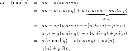
and

and thus |γ(n)|{0,…,p - 1}. Since an (mod p) {0,…,p - 1} evaluating δ(n) is
unnecessary, because δ(n) = 0 iff γ(n) ≥ 0 and δ(n) = 1 iff γ(n) < 0. This leads to the
following algorithm:
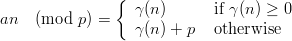
q and r can be precomputed, calculating (ndiv q) and (n mod q) requires on some computers only one instruction, so this is a very efficient algorithm.
For the usual choice of 231 - 1 for p the above can be applied for all a < 215. If p is smaller than that, then the limitation that all intermediate results should be between -p and p is unnecessarily tight. On a b-bit computer all integers between -2b-1 and 2b-1 (exclusive) are representable. If we loosen the restriction on a from a2 < p to a2 < 2b-2, the term r (ndiv q) is no longer bounded by p. But it can be shown that 2b-1 is an upper bound:
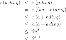
The while loop can execute at most ⌈2b-1∕p⌉ times. L’Ecuyer and Côté [56] observed that in the average case very few iterations are executed, thus this algorithm is efficient.
If a is not restricted in any way (except of course by the requirement a < p) one can use decomposition to reduce the multiplication to cases for which we already have solutions. This can be achieved by writing a in base 2d, where d = (b - 2)∕2 (usually 15 on current 32-bit computers):
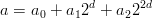
with 0 ≤ a0,a1 < 2d, and a
2 {0, 1}. Then
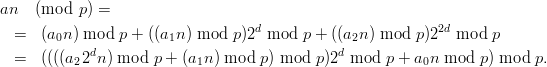
|
Modular addition is simple to solve, though it is not trivial. A straightforward implementation might look like this:
This is correct, as long as a + b is still fully representable with the data type used. Assuming that the usual signed integer type is used, an overflow would occur if a + b is negative. It cannot happen that a + b is positive in spite of an overflow, since a and b are both smaller than 2b-1 - 1 (assuming a b-bit computer) and (2b-1 - 1) + 1 wraps to -2b-1. If we detect an overflow, subtracting p will bring the result back into the interval [0,p - 1]. Thus this
is a correct implementation.
Let us quickly summarize the main points of this thesis.
Let p be a (large) prime and a,b,n0 ℤp. The explicit inversive congruential
generator (abbreviated as “EICG”) with parameters p,a,b, and n0 defines
a sequence (yn)n≥0 in ℤp by

and a sequence eicg(p,a,b,n0) = (xn)n≥0 of pseudorandom numbers in [0, 1[ by
where c denotes the multiplicative inverse modulo p extended by 0 := 0.
 . Examining tuples formed using the full period of the
EICG we get Dp(s) = (p-1∕2(log p)s) as an upper bound, and an existence
statement which implies that this bound is the best possible up to the
logarithmic factor.
. Examining tuples formed using the full period of the
EICG we get Dp(s) = (p-1∕2(log p)s) as an upper bound, and an existence
statement which implies that this bound is the best possible up to the
logarithmic factor.
For parts of the period we get similar results: as an upper bound we
have DN(s) = (N-1p1∕2(log p)s+1), and we can show the existence of
EICGs with DN(s) ≥ cN-1∕2 for some constant c.
[1] S.L. Anderson. Random number generators on vector supercomputers and other advanced architectures. SIAM Rev., 32:221–251, 1990.
[2] D.A. André, G.L. Mullen, and H. Niederreiter. Figures of merit for digital multistep pseudorandom numbers. Math. Comp., 54:737–748, 1990.
[3] K. Binder and D.W. Heermann. Monte Carlo Simulation in Statistical Physics. An Introduction. 2nd corr. ed. Springer-Verlag Heidelberg New York, 1992.
[4] P. Bratley, B. L. Fox, and L. E. Schrage. A Guide to Simulation. Springer Verlag, second edition, 1987.
[5] G.J. Chaitin. Randomness and mathematical proof. Sci. Amer., 232:47–52, 1975.
[6] Wun-Seng Chou. On inversive maximal period polynomials over finite fields. Appl. Algebra Engrg. Comm. Comput., 6:245–250, 1995.
[7] T. Cochrane. On a trigonometric inequality of Vinogradov. J. Number Th., 27:9–16, 1987.
[8] Thomas H. Corman, Charles E. Leiserson, and Ronald L. Rivest. Introduction to Algorithms. The MIT Press, first edition, 1989.
[9] R.R. Coveyou and R.D. MacPherson. Fourier analysis of uniform random number generators. J. Assoc. Comput. Mach., 14:100–119, 1967.
[10] A. De Matteis and S. Pagnutti. Parallelization of random number generators and long-range correlations. Numer. Math., 53:595–608, 1988.
[11] G. Dueck and T. Scheuer. Threshold Accepting: A General Purpose Algorithm Appearing Superior to Simulated Annealing. Journal of Computational Physics, pages 161–175, 1990.
[12] W.F. Eddy. Random number generators for parallel processors. J. Comp. Appl. Math., 31:63–71, 1990.
[13] J. Eichenauer, H. Grothe, and J. Lehn. Marsaglia’s lattice test and non-linear congruential pseudo random number generators. Metrika, 35:241–250, 1988.
[14] J. Eichenauer and J. Lehn. A non-linear congruential pseudo random number generator. Statist. Papers, 27:315–326, 1986.
[15] J. Eichenauer-Herrmann. Statistical independence of a new class of inversive congruential pseudorandom numbers. Math. Comp., 60:375–384, 1993.
[16] J. Eichenauer-Herrmann. Nonoverlapping pairs of explicit inversive congruential pseudorandom numbers. Monatsh. Math., 119:49–61, 1995.
[17] J. Eichenauer-Herrmann. Modified explicit inversive congruential pseudorandom numbers with power of 2 modulus. Statistics and Computing, 6:31–36, 1996.
[18] J. Eichenauer-Herrmann and F. Emmerich. A review of compound methods for pseudorandom number generation. In P. Hellekalek, G. Larcher, and P. Zinterhof, editors, Proceedings of the 1st Salzburg Minisymposium on Pseudorandom Number Generation and Quasi-Monte Carlo Methods, Salzburg, Nov 18, 1994, volume ACPC/TR 95-4 of Technical Report Series, pages 5–14. ACPC – Austrian Center for Parallel Computation, University of Vienna, Austria, 1995.
[19] J. Eichenauer-Herrmann and F. Emmerich. Compound inversive congruential numbers: an average-case analysis. Math. Comp., to appear, 65:215–225, 1996.
[20] J. Eichenauer-Herrmann and H. Grothe. A remark on long-range correlations in multiplicative congruential pseudo random number generators. Numer. Math., 56:609–611, 1989.
[21] J. Eichenauer-Herrmann and E. Herrmann. A survey of quadratic and inversive congruential pseudorandom numbers. Submitted to Proceedings of the Second International Conference on Monte Carlo and Quasi-Monte Carlo Methods in Scientific Computing, Salzburg, July 9–12, 1996.
[22] J. Eichenauer-Herrmann and K. Ickstadt. Explicit inversive congruential pseudorandom numbers with power of two modulus. Math. Comp., 62:787–797, 1994.
[23] J. Eichenauer-Herrmann and H. Niederreiter. Bounds for exponential sums and their applications to pseudorandom numbers. Acta Arith., 67:269–281, 1994.
[24] K. Entacher. Selected random number generators in run tests. Preprint, Institut für Mathematik, Universität Salzburg, Austria, 1996.
[25] K. Entacher and P. Hellekalek. Parallel stochastic simulation: inversive pseudorandom number generators. In G. De Pietro and P. Zinterhof A. Giordano, M. Vajteršic, editors, Proceedings of the International Workshop Parallel Numerics 95, Sorrento, Italy, September 27–29, 1995, pages 1–14. IRSIP Institute of the NRC of Italy, Naples, 1995.
[26] K. Entacher and H. Leeb. Inversive pseudorandom number generators: empirical results. In Proceedings of the Conference Parallel Numerics 95, Sorrento, Italy, September 27–29, 1995, 1995.
[27] G.S. Fishman. Multiplicative congruential random number generators with modulus 2β: an exhaustive analysis for β = 32 and a partial analysis for β = 48. Math. Comp., 54:331–344, 1990.
[28] G.S. Fishman and L.R. Moore. A statistical evaluation of multiplicative congruential random number generators with modulus 231 - 1. J. Amer. Statist. Assoc., 77:129–136, 1982.
[29] G.S. Fishman and L.R. Moore. An exhaustive analysis of multiplicative congruential random number generators with modulus 231 -1. SIAM J. Sci. Statist. Comput. (see also the Erratum, ibid. 7(1986), p. 1058), 7:24–45, 1986.
[30] M. Flahive and H. Niederreiter. On inversive congruential generators for pseudorandom numbers. In G.L. Mullen and P.J.-S. Shiue, editors, Finite Fields, Coding Theory, and Advances in Communications and Computing, pages 75–80. Dekker, New York, 1992.
[31] Mark Fleischer. Simulated Annealing: Past, Present, and Future. In Proceedings of the 1995 Winter Simulation Conference, pages 155–161, 1995.
[32] J. Foley, A. van Dam, S. Feiner, and J. Hughes. Computer Graphics: Principles and Practice. Addison-Wesley, second edition, 1990.
[33] I. Goldberg and D. Wagner. Netscape SSL implementation cracked!
Available on the WWW at
http://tezcat.com/web/security/items/ssl-news.txt.
[34] T. Gonzales, S. Sahni, and W.R. Franta. An efficient algorithm for the Kolmogorov-Smirnov and Lillefors tests. ACM Trans. Mathem. Softw., 3:60–64, 1977.
[35] J. Gordon. Fast Multiplicative Inverse in Moduar Arithmetic. In H. J. Beker and F. S. Piper, editors, Cryptography and Coding. Oxford Clarendon Press, 1989.
[36] J.H. Halton. Pseudo-random trees: multiple independent sequence generators for parallel and branching computations. J. Comp. Physics, 84:1–56, 1989.
[37] F. Härtel. Zufallszahlen für Simulationsmodelle. PhD thesis, Hochschule St. Gallen für Wirtschafts-, Rechts- und Sozialwissenschaften, St. Gallen, 1994.
[38] S. Heinrich. Efficient algorithms for computing the L2 discrepancy. Interner Bericht, Fachbereich Informatik, Universität Kaiserslautern, 1995.
[39] P. Hellekalek. Study of algorithms for primitive polynomials. Report D5H-1, CEI-PACT Project, WP5.1.2.1.2, Research Institute for Software Technology, University of Salzburg, Austria, 1994.
[40] P. Hellekalek. Correlations between pseudorandom numbers: theory and numerical practice. In P. Hellekalek, G. Larcher, and P. Zinterhof, editors, Proceedings of the 1st Salzburg Minisymposium on Pseudorandom Number Generation and Quasi-Monte Carlo Methods, Salzburg, Nov 18, 1994, volume ACPC/TR 95-4 of Technical Report Series, pages 43–73. ACPC – Austrian Center for Parallel Computation, University of Vienna, Austria, 1995.
[41] P. Hellekalek. On correlation analysis of pseudorandom numbers. Submitted to Proceedings of the Second International Conference on Monte Carlo and Quasi-Monte Carlo Methods in Scientific Computing, Salzburg, July 9–12, 1996, 1996.
[42] P. Hellekalek and K. Entacher. Revised implementation and testing of the algorithms for IMP-polynomials. Report D5H-3, CEI-PACT Project, WP5.1.2.1.2, Research Institute for Software Technology, University of Salzburg, Austria, 1995.
[43] P. Hellekalek and K. Entacher. Tables of IMP-polynomials. Report D5H-4, CEI-PACT Project, WP5.1.2.1.2, Research Institute for Software Technology, University of Salzburg, Austria, 1995.
[44] P. Hellekalek and H. Leeb. Dyadic diaphony. To appear in Acta Arithmetica, 1996.
[45] P. Hellekalek, M. Mayer, and A. Weingartner. Implementation of algorithms for IMP-polynomials. Report D5H-2, CEI-PACT Project, WP5.1.2.1.2, Research Institute for Software Technology, University of Salzburg, Austria, 1994.
[46] P. Hellekalek and H. Niederreiter. The weighted spectral test: diaphony. In preparation, 1996.
[47] F. James, J. Hoogland, and R. Kleiss. Multidimensional sampling for simulation and integration: measures, discrepancies, and quasi-random numbers. Preprint submitted to Computer Physics Communications, 1996.
[48] M.H. Kalos and P.A. Whitlock. Monte Carlo Methods, Volume I: Basics. Wiley, New York, 1986.
[49] J. Kiefer. On large deviations of the empiric d.f. of vector chance variables and a law of the iterated logarithm. Pacific J. Math., 11:649–660, 1961.
[50] D. E. Knuth. The Art of Computer Programming, Vol. 2: Seminumerical Algorithms. Addison-Wesley, Reading, MA, second edition, 1981.
[51] L. Kuipers and H. Niederreiter. Uniform Distribution of Sequences. Wiley and Sons, New York London Sydney Toronto, 1974.
[52] J. C. Lagarias. Pseudorandom numbers. Statistical Science, 8:31–39, 1993.
[53] P. L’Ecuyer. Random numbers for simulation. Comm. ACM, 33:85–97, 1990.
[54] P. L’Ecuyer. Testing random number generators. In J.J. Swain et al., editor, Proc. 1992 Winter Simulation Conference (Arlington, Va., 1992), pages 305–313. IEEE Press, Piscataway, N.J., 1992.
[55] P. L’Ecuyer. Uniform random number generation. Ann. Oper. Res., 53:77–120, 1994.
[56] P. L’Ecuyer and S. Côté. Implementing a Random Number Package with Splitting Facilities. ACM Transactions on Mathematical Software, 17(1):98–111, March 1991.
[57] H. Leeb. pLab – a system for testing random numbers. In M. Vajteršic and P. Zinterhof, editors, Proceedings of the International Workshop on Parallel Numerics ’94, Smolenice, Sept. 19–21, pages 89–99. Slovak Academy of Sciences, Institute for Informatics, 1994. Available on the internet at http://random.mat.sbg.ac.at.
[58] H. Leeb. On the digit test. In P. Hellekalek, G. Larcher, and P. Zinterhof, editors, Proceedings of the 1st Salzburg Minisymposium on Pseudorandom Number Generation and Quasi-Monte Carlo Methods, Salzburg, Nov 18, 1994, volume ACPC/TR 95-4 of Technical Report Series, pages 109–121. ACPC – Austrian Center for Parallel Computation, University of Vienna, Austria, 1995.
[59] H. Leeb. Random Numbers for Computer Simulation. Master’s thesis, Institut für Mathematik, Universität Salzburg, Austria, 1995.
[60] H. Leeb. A weak law for diaphony. Rist++ 13, Research Institute for Software Technology, University of Salzburg, 1996.
[61] H. Leeb and S. Wegenkittl. Inversive and linear congruential pseudorandom number generators in empirical tests. submitted to ACM Trans. Modeling and Computer Simulation, 1996.
[62] V. F. Lev. On two versions of L2-discrepancy and geometrical interpretation of diaphony. Acta Math. Hungar., 69:281–300, 1995.
[63] H. Levene and J. Wolfowitz. The covariance matrix of runs up and down. Annals Math. Stat., 15 :59–69, 1944.
[64] R. Lidl and H. Niederreiter. Finite Fields. Addison-Wesley, Reading, Mass., 1983.
[65] G. Marsaglia. Random numbers fall mainly in the planes. Proc. Nat. Acad. Sci., 61:25–28, 1968.
[66] G. Marsaglia. A current view of random number generators. In L. Brillard, editor, Computer Science and Statistics: The Interface, pages 3–10, Amsterdam, 1985. Elsevier Science Publishers B.V. (North Holland).
[67] L. Ming and P. Vitány. An Introduction To Kolmogorov Complexity And Its Applications. Texts and Monographs in Computer Science. Springer Verlag, New York, 1993.
[68] C.J. Moreno and O. Moreno. Exponential sums and Goppa codes: I. Proc. Amer. Math. Soc., 111:523–531, 1991.
[69] Netscape Communications Corporation. Potential Vulnerability in
Netscape Products. Available on the WWW at
http://www.netscape.com/newsref/std/random_seed_security.html.
[70] H. Niederreiter. Random Number Generation and Quasi-Monte Carlo Methods. SIAM, Philadelphia, USA, 1992.
[71] H. Niederreiter. On a new class of pseudorandom numbers for simulation methods. J. Comput. Appl. Math., 56:159–167, 1994.
[72] H. Niederreiter. New developments in uniform pseudorandom number and vector generation. In H. Niederreiter and P.J.-S. Shiue, editors, Monte Carlo and Quasi-Monte Carlo Methods in Scientific Computing, volume 106 of Lecture Notes in Statistics. Springer-Verlag, Heidelberg New York, 1995.
[73] S.K. Park and K.W. Miller. Random number generators: good ones are hard to find. Comm. ACM, 31:1192–1201, 1988.
[74] C. A. Pickover. Random number generators: pretty good ones are easy to find. The Visual Computer, 11:369–377, 1995.
[75] B. D. Ripley. Stochastic Simulation. John Wiley, New York, 1987.
[76] R. A. Rueppel. Stream Ciphers. In Gustavus J. Simmons, editor, Contemporary cryptology: the science of information integrity, chapter 2. IEEE Press, 1992.
[77] Bruce Schneier. Applied Cryptography. John Wiley & Sons, Inc., first edition, 1993.
[78] I.M. Sobol. Die Monte-Carlo-Methode. VEB Deutscher Verlag der Wissenschaften, 1983.
[79] H. Stegbuchner. Zur quantitativen Theorie der Gleichverteilung mod 1. Arbeitsberichte, Mathematisches Institut der Universität Salzburg, Salzburg, Austria, 1980.
[80] O. Strauch. L2 discrepancy. Math. Slovaca, 44:601–632, 1994.
[81] R.C. Tausworthe. Random numbers generated by linear recurrence modulo two. Math. Comp., 19:201–209, 1965.
[82] S. Tezuka. Uniform Random Numbers: Theory and Practice. Kluwer Academic Publ., 1995.
[83] S. Tezuka and M. Fushimi. Calculation of Fibonacci polynomials for GFSR sequences with low discrepancies. Math. Comp., 60:763–770, 1993.
[84] J.F. Traub and H. Woźniakowski. The Monte Carlo algorithm with a pseudorandom generator. Math. Comp., 58:323–339, 1992.
[85] S. Wegenkittl. Empirical Testing of Pseudorandom Number Generators. Master’s thesis, Institut für Mathematik, Universität Salzburg, Austria, 1995.
[86] S. Wegenkittl. On empirical testing of pseudorandom number generators. In G. De Pietro, A. Giordano, M. Vajteršic, and P. Zinterhof, editors, Proceedings of the International Workshop Parallel Numerics 95, Sorrento, Italy, September 27–29, 1995, pages 113–123. IRSIP Institute of the NRC of Italy, Naples, 1995.
[87] A. Weingartner. Nonlinear congruential pseudorandom number generators. Master’s thesis, Universität Salzburg, Austria, 1994.
[88] B.A. Wichmann and I.D. Hill. An efficient and portable pseudo-random number generator. Appl. Statist., 31:188–190, 1982. Corrections, ibid. 33, 123 (1994).
[89] P. Winker and Kai-Tai Fang. Application of threshold accepting to the evaluation of the discrepancy of a set of points. Research report, Universität Konstanz, Germany, 1995.
[90] P. Zinterhof. Über einige Abschätzungen bei der Approximation von Funktionen mit Gleichverteilungsmethoden. Sitzungsber. Österr. Akad. Wiss. Math.-Natur. Kl. II, 185:121–132, 1976.
Name: Otmar Lendl
Date of birth: May 8th, 1970
Place of birth: Salzburg, Austria
Parents: Ingeborg and Wolfgang Lendl
Education:
| 1976–1980: | Volksschule in Salzburg |
| 1980–1988: | Gymnasium in Salzburg |
| 1988–1996: | University studies (M.Sc. in Mathematics) |
| at the University of Salzburg |